SQL Guide: How to Write Queries Better (Part 2)
Continued article SQL Guide: How to Write Queries Better (Part 1)
 Knowing that antipatterns are not static and evolve as you grow as a SQL developer, and the fact that there are many things to keep in mind when thinking about alternatives also means that avoiding antipatterns and rewriting queries can be quite difficult task. Any help can come in handy, which is why a more structured approach to query optimization using some tools may be most effective.
It should also be noted that some of the antipatterns mentioned in the last section are rooted in performance issues, such as the
,
and
operators and their absence when using indices. Thinking about performance requires not only a more structured, but also a deeper approach.
However, this structured and in-depth approach will mainly be based on the query plan, which, as you recall, is the result of a query first parsed into a “parse tree” or “parse tree” and determines exactly which algorithm used for each operation and how their execution is coordinated.
As you read in the introduction, you may need to check and set up plans that are manually compiled by the optimizer. In such cases, you will need to analyze your request again by looking at the request plan.
To access this plan, you must use the tools provided by the database management system. The following tools may be at your disposal:
Please note that when working with PostgreSQL, you can make a distinction between
, where you simply get a description that tells how the planner intends to execute the query without executing it, while
actually executes the query and returns you the analysis expected and actual request plans. Generally speaking, a real execution plan is a plan in which the request is actually executed, while an evaluation execution plan determines what it will do without fulfilling the request. Although this is logically equivalent, the actual execution plan is much more useful as it contains additional information and statistics about what really happened when the request was executed.
In the rest of this section, you will learn more about
and
, and how to use them to get more information about the query plan and its possible performance. To do this, start with a few examples in which you will work with two tables:
and
.
You can get the current information from the
table using
; Be sure to place it directly above the request, and after executing it, it will return the query plan to you:
In this case, you see that the cost of the request is
, and the number of rows is
. The width of the number of columns is
.
In addition, you can update statistics using
.
Besides
and
, you can also get the actual runtime with
:
The disadvantage of using
is that the query is actually executed, so be careful with this!
So far, all the algorithms that you have seen are
(Sequential Scan) or Full Table Scan: this is a scan performed in a database where each row of the scanned table is read in serial order and the columns found are checked for compliance with the condition or not. In terms of performance, sequential scans are certainly not the best execution plan because you are still doing a full table scan. However, this is not so bad when the table does not fit in memory: sequential reads are pretty fast even on slow disks.
You will learn more about this later when we talk about index scan.
However, there are other algorithms. Take, for example, this query plan for a connection:
You see that the query optimizer chose
here! Remember this operation, as you will need it to assess the time complexity of your request. For now, note that there is no index in
, which we add in the following example:
You see that by creating the index, the query optimizer has now decided to use
when scanning the
index.
Note the difference between index scanning and full table scanning or sequential scanning: the first, also called “table scanning”, scans the data or index pages to find the corresponding records, while the second scans each row of the table.
You see that the overall runtime has decreased and performance should be better, but there are two index scans, which makes memory more important here, especially if the table does not fit into it. In such cases, you must first perform a full index scan, which is performed using fast sequential reads and is not a problem, but then you have many random read operations to select rows by index value. These are random read operations that are usually several orders of magnitude slower than sequential ones. In these cases, a full table scan does indeed happen faster than a full index scan.
Tip: If you want to learn more about EXPLAIN or consider examples in more detail, consider reading Guillaume Lelarge ’s Understanding Explain .
Now that you’ve briefly reviewed the query plan, you can start digging deeper and think about performance in more formal terms using the theory of computational complexity. This is a field of theoretical computer science, which, among other things, focuses on the classification of computational problems depending on their complexity; These computational problems may be algorithms, but also queries.
However, for queries, they are not necessarily classified according to their complexity, but rather, depending on the time required to complete them and obtain results. This is called time complexity, and you can use the big O notation to formulate or measure this type of complexity.
With the designation big O, you express the runtime in terms of how fast it grows relative to the input, as the input becomes arbitrarily large. The large O notation excludes coefficients and members of a lower order, so you can focus on the important part of the execution time of your query: its growth rate. When expressed in this way, discarding the coefficients and terms of a lower order, they say that the time complexity is described asymptotically. This means that the input size goes to infinity.
In a database language, complexity determines how long it takes to complete a query as the size of the data tables and therefore the database grows.
Please note that the size of your database increases not only from the increase in the amount of data in the tables, but the fact that there are indexes also plays a role in size.
Estimating the time complexity of your query plan
As you saw earlier, the execution plan, among other things, determines which algorithm is used for each operation, which allows you to logically express each query execution time as a function of the size of the table included in the query plan, which is called the complexity function. In other words, you can use the big O notation and the execution plan to evaluate query complexity and performance.
In the following sections, you will get an overview of the four types of time complexity, and you will see some examples of how the time complexity of requests can vary depending on the context in which it is executed.
Hint: indexes are part of this story!
However, it should be noted that there are different types of indexes, different execution plans, and different implementations for different databases, so the temporary difficulties listed below are very general and may vary depending on specific settings.
They say that an algorithm works in constant time if it needs the same amount of time regardless of the size of the input data. When it comes to a query, it will be executed in constant time if the same amount of time is required regardless of the size of the table.
This type of query is not really common, but here is one such example:
The time complexity is constant, since one arbitrary row is selected from the table. Therefore, the length of time should not depend on the size of the table.
They say that the algorithm works in linear time, if its execution time is directly proportional to the size of the input data, that is, the time increases linearly with the size of the input data. For databases, this means that the execution time will be directly proportional to the size of the table: as the number of rows in the table grows, the query execution time increases.
An example is a query with a
for an unindexed column: a full table scan or
will be required, which will lead to O (n) time complexity. This means that each line must be read in order to find the line with the desired identifier (ID). You do not have any restrictions at all, so you need to count every line, even if the first line matches the condition.
Consider also the following example query, which will have O (n) complexity if there is no index on the
field:
The linear runtime is closely related to the runtime of plans that have table joins. Here are some examples:
Remember: a nested join is a join that compares each record in one table with each record in another.
It is said that an algorithm works in logarithmic time if its execution time is proportional to the logarithm of the input size; For queries, this means that they will be executed if the execution time is proportional to the logarithm of the database size.
This logarithmic time complexity is valid for query plans where
or clustered index scans. A clustered index is an index where the final level of the index contains the actual rows of the table. A clustered index is similar to any other index: it is defined in one or more columns. They form the index key. The clustering key is the key columns of a clustered index. Scanning a clustered index is basically the operation of reading your DBMS for a row or rows from top to bottom in a clustered index.
Consider the following query example, where there is an index for
and which usually results in O (log (n)) complexity:
Note that without an index, the time complexity would be O (n).
It is believed that the algorithm is executed in quadratic time, if its execution time is proportional to the square of the input size. Again, for databases, this means that the query execution time is proportional to the square of the database size.
A possible example of a quadratic time complexity query is the following:
The minimum complexity may be O (n log (n)), but the maximum complexity may be O (n ^ 2) based on the connection attribute index information.
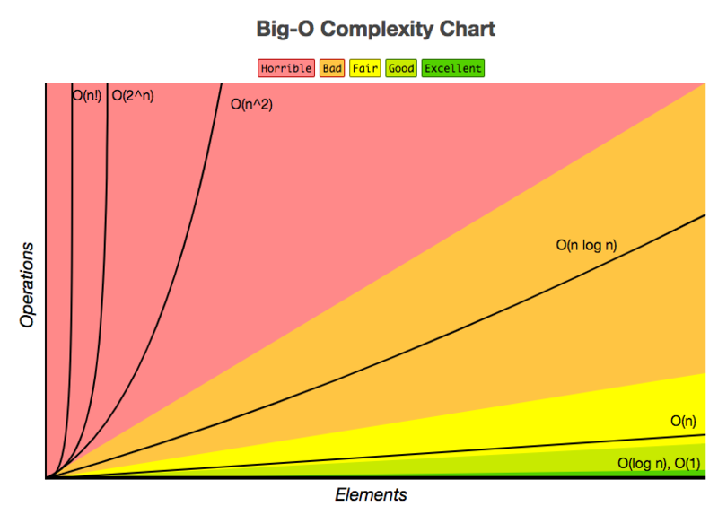
To summarize, you can also take a look at the following cheat sheet to evaluate query performance based on their time complexity and their effectiveness:
Given the query execution plan and time complexity, you can further customize your SQL query. You can start by focusing on the following points:
Congratulations! You have come to the end of this article, which just gave you a small look at the performance of SQL queries. I hope you have more information about antipatterns, the query optimizer, and the tools you can use to analyze, evaluate, and interpret the complexity of your query plan. However, you still have so much to discover! If you want to know more, read the book “Database Management Systems” by R. Ramakrishnan and J. Gehrke.
Finally, I do not want to deny StackOverflow from you in this quote:
From request to execution plans
Knowing that antipatterns are not static and evolve as you grow as a SQL developer, and the fact that there are many things to keep in mind when thinking about alternatives also means that avoiding antipatterns and rewriting queries can be quite difficult task. Any help can come in handy, which is why a more structured approach to query optimization using some tools may be most effective.
It should also be noted that some of the antipatterns mentioned in the last section are rooted in performance issues, such as the
AND
,
OR
and
NOT
operators and their absence when using indices. Thinking about performance requires not only a more structured, but also a deeper approach.
However, this structured and in-depth approach will mainly be based on the query plan, which, as you recall, is the result of a query first parsed into a “parse tree” or “parse tree” and determines exactly which algorithm used for each operation and how their execution is coordinated.
Query optimization
As you read in the introduction, you may need to check and set up plans that are manually compiled by the optimizer. In such cases, you will need to analyze your request again by looking at the request plan.
To access this plan, you must use the tools provided by the database management system. The following tools may be at your disposal:
- Some packages contain tools that generate a graphical representation of the query plan. Consider the following example:

- Other tools will provide a textual description of the query plan. One example is the
EXPLAIN PLAN
statement in Oracle, but the name of the instruction depends on the DBMS you are working with. Elsewhere you can findEXPLAIN
(MySQL, PostgreSQL) orEXPLAIN QUERY PLAN
(SQLite).
Please note that when working with PostgreSQL, you can make a distinction between
EXPLAIN
, where you simply get a description that tells how the planner intends to execute the query without executing it, while
EXPLAIN ANALYZE
actually executes the query and returns you the analysis expected and actual request plans. Generally speaking, a real execution plan is a plan in which the request is actually executed, while an evaluation execution plan determines what it will do without fulfilling the request. Although this is logically equivalent, the actual execution plan is much more useful as it contains additional information and statistics about what really happened when the request was executed.
In the rest of this section, you will learn more about
EXPLAIN
and
ANALYZE
, and how to use them to get more information about the query plan and its possible performance. To do this, start with a few examples in which you will work with two tables:
one_million
and
half_million
.
You can get the current information from the
one_million
table using
EXPLAIN
; Be sure to place it directly above the request, and after executing it, it will return the query plan to you:
EXPLAIN SELECT * FROM one_million; QUERY PLAN ____________________________________________________ Seq Scan on one_million (cost=0.00..18584.82 rows=1025082 width=36) (1 row)
In this case, you see that the cost of the request is
0.00..18584.82
, and the number of rows is
1025082
. The width of the number of columns is
36
.
In addition, you can update statistics using
ANALYZE
.
ANALYZE one_million; EXPLAIN SELECT * FROM one_million; QUERY PLAN ____________________________________________________ Seq Scan on one_million (cost=0.00..18334.00 rows=1000000 width=37) (1 row)
Besides
EXPLAIN
and
ANALYZE
, you can also get the actual runtime with
EXPLAIN ANALYZE
:
EXPLAIN ANALYZE SELECT * FROM one_million; QUERY PLAN ___________________________________________________________ Seq Scan on one_million (cost=0.00..18334.00 rows=1000000 width=37) (actual time=0.015..1207.019 rows=1000000 loops=1) Total runtime: 2320.146 ms (2 rows)
The disadvantage of using
EXPLAIN ANALYZE
is that the query is actually executed, so be careful with this!
So far, all the algorithms that you have seen are
Seq Scan
(Sequential Scan) or Full Table Scan: this is a scan performed in a database where each row of the scanned table is read in serial order and the columns found are checked for compliance with the condition or not. In terms of performance, sequential scans are certainly not the best execution plan because you are still doing a full table scan. However, this is not so bad when the table does not fit in memory: sequential reads are pretty fast even on slow disks.
You will learn more about this later when we talk about index scan.
However, there are other algorithms. Take, for example, this query plan for a connection:
EXPLAIN ANALYZE SELECT * FROM one_million JOIN half_million ON (one_million.counter=half_million.counter); QUERY PLAN _________________________________________________________________ Hash Join (cost=15417.00..68831.00 rows=500000 width=42) (actual time=1241.471..5912.553 rows=500000 loops=1) Hash Cond: (one_million.counter = half_million.counter) -> Seq Scan on one_million (cost=0.00..18334.00 rows=1000000 width=37) (actual time=0.007..1254.027 rows=1000000 loops=1) -> Hash (cost=7213.00..7213.00 rows=500000 width=5) (actual time=1241.251..1241.251 rows=500000 loops=1) Buckets: 4096 Batches: 16 Memory Usage: 770kB -> Seq Scan on half_million (cost=0.00..7213.00 rows=500000 width=5) (actual time=0.008..601.128 rows=500000 loops=1) Total runtime: 6468.337 ms
You see that the query optimizer chose
Hash Join
here! Remember this operation, as you will need it to assess the time complexity of your request. For now, note that there is no index in
half_million.counter
, which we add in the following example:
CREATE INDEX ON half_million(counter); EXPLAIN ANALYZE SELECT * FROM one_million JOIN half_million ON (one_million.counter=half_million.counter); QUERY PLAN ________________________________________________________________ Merge Join (cost=4.12..37650.65 rows=500000 width=42) (actual time=0.033..3272.940 rows=500000 loops=1) Merge Cond: (one_million.counter = half_million.counter) -> Index Scan using one_million_counter_idx on one_million (cost=0.00..32129.34 rows=1000000 width=37) (actual time=0.011..694.466 rows=500001 loops=1) -> Index Scan using half_million_counter_idx on half_million (cost=0.00..14120.29 rows=500000 width=5) (actual time=0.010..683.674 rows=500000 loops=1) Total runtime: 3833.310 ms (5 rows)
You see that by creating the index, the query optimizer has now decided to use
Merge join
when scanning the
Index Scan
index.
Note the difference between index scanning and full table scanning or sequential scanning: the first, also called “table scanning”, scans the data or index pages to find the corresponding records, while the second scans each row of the table.
You see that the overall runtime has decreased and performance should be better, but there are two index scans, which makes memory more important here, especially if the table does not fit into it. In such cases, you must first perform a full index scan, which is performed using fast sequential reads and is not a problem, but then you have many random read operations to select rows by index value. These are random read operations that are usually several orders of magnitude slower than sequential ones. In these cases, a full table scan does indeed happen faster than a full index scan.
Tip: If you want to learn more about EXPLAIN or consider examples in more detail, consider reading Guillaume Lelarge ’s Understanding Explain .
Time Complexity and Big O
Now that you’ve briefly reviewed the query plan, you can start digging deeper and think about performance in more formal terms using the theory of computational complexity. This is a field of theoretical computer science, which, among other things, focuses on the classification of computational problems depending on their complexity; These computational problems may be algorithms, but also queries.
However, for queries, they are not necessarily classified according to their complexity, but rather, depending on the time required to complete them and obtain results. This is called time complexity, and you can use the big O notation to formulate or measure this type of complexity.
With the designation big O, you express the runtime in terms of how fast it grows relative to the input, as the input becomes arbitrarily large. The large O notation excludes coefficients and members of a lower order, so you can focus on the important part of the execution time of your query: its growth rate. When expressed in this way, discarding the coefficients and terms of a lower order, they say that the time complexity is described asymptotically. This means that the input size goes to infinity.
In a database language, complexity determines how long it takes to complete a query as the size of the data tables and therefore the database grows.
Please note that the size of your database increases not only from the increase in the amount of data in the tables, but the fact that there are indexes also plays a role in size.
Estimating the time complexity of your query plan
As you saw earlier, the execution plan, among other things, determines which algorithm is used for each operation, which allows you to logically express each query execution time as a function of the size of the table included in the query plan, which is called the complexity function. In other words, you can use the big O notation and the execution plan to evaluate query complexity and performance.
In the following sections, you will get an overview of the four types of time complexity, and you will see some examples of how the time complexity of requests can vary depending on the context in which it is executed.
Hint: indexes are part of this story!
However, it should be noted that there are different types of indexes, different execution plans, and different implementations for different databases, so the temporary difficulties listed below are very general and may vary depending on specific settings.
O (1): Constant Time
They say that an algorithm works in constant time if it needs the same amount of time regardless of the size of the input data. When it comes to a query, it will be executed in constant time if the same amount of time is required regardless of the size of the table.
This type of query is not really common, but here is one such example:
SELECT TOP 1 t.* FROM t
The time complexity is constant, since one arbitrary row is selected from the table. Therefore, the length of time should not depend on the size of the table.
Linear Time: O (n)
They say that the algorithm works in linear time, if its execution time is directly proportional to the size of the input data, that is, the time increases linearly with the size of the input data. For databases, this means that the execution time will be directly proportional to the size of the table: as the number of rows in the table grows, the query execution time increases.
An example is a query with a
WHERE
for an unindexed column: a full table scan or
Seq Scan
will be required, which will lead to O (n) time complexity. This means that each line must be read in order to find the line with the desired identifier (ID). You do not have any restrictions at all, so you need to count every line, even if the first line matches the condition.
Consider also the following example query, which will have O (n) complexity if there is no index on the
i_id
field:
SELECT i_id FROM item;
- The previous one also means that other queries, such as queries for calculating the number of rows
COUNT (*) FROM TABLE;
will have O (n) time complexity, since a full table scan will be required because the total number of rows has not been saved for the table. Otherwise, the time complexity would be similar to O (1) .
The linear runtime is closely related to the runtime of plans that have table joins. Here are some examples:
- Hash join has the expected complexity of O (M + N). The classic hash join algorithm for internally joining two tables first prepares the hash table of the smaller table. Hash table entries consist of a connection attribute and its string. The hash table is accessed by applying the hash function to the connection attribute. Once the hash table is built, a large table is scanned, and the corresponding rows from the smaller table are found by searching the hash table.
- Merge joins usually have O (M + N) complexity, but it will depend heavily on the join column indices and, if there is no index, on whether the rows are sorted according to the keys used in the join:
- If both tables are sorted according to the keys used in the join, then the query will have a time complexity of O (M + N).
- If both tables have an index for joined columns, then the index already supports these columns in order and sorting is not required. The difficulty will be O (M + N).
- If none of the tables has an index on connected columns, you must first sort both tables so that the complexity will look like O (M log M + N log N).
- If only one of the tables has an index on the connected columns, then only the table that does not have an index must be sorted before the join step occurs, so that the complexity will look like O (M + N log N).
- For nested joins, the complexity is usually O (MN). This join is effective when one or both tables are extremely small (for example, less than 10 records), which is a very common situation when evaluating queries, since some subqueries are written to return only one row.
Remember: a nested join is a join that compares each record in one table with each record in another.
Logarithmic Time: O (log (n))
It is said that an algorithm works in logarithmic time if its execution time is proportional to the logarithm of the input size; For queries, this means that they will be executed if the execution time is proportional to the logarithm of the database size.
This logarithmic time complexity is valid for query plans where
Index Scan
or clustered index scans. A clustered index is an index where the final level of the index contains the actual rows of the table. A clustered index is similar to any other index: it is defined in one or more columns. They form the index key. The clustering key is the key columns of a clustered index. Scanning a clustered index is basically the operation of reading your DBMS for a row or rows from top to bottom in a clustered index.
Consider the following query example, where there is an index for
i_id
and which usually results in O (log (n)) complexity:
SELECT i_stock FROM item WHERE i_id = N;
Note that without an index, the time complexity would be O (n).
Quadratic Time: O (n ^ 2)
It is believed that the algorithm is executed in quadratic time, if its execution time is proportional to the square of the input size. Again, for databases, this means that the query execution time is proportional to the square of the database size.
A possible example of a quadratic time complexity query is the following:
SELECT * FROM item, author WHERE item.i_a_id=author.a_id
The minimum complexity may be O (n log (n)), but the maximum complexity may be O (n ^ 2) based on the connection attribute index information.
To summarize, you can also take a look at the following cheat sheet to evaluate query performance based on their time complexity and their effectiveness:
SQL tuning
Given the query execution plan and time complexity, you can further customize your SQL query. You can start by focusing on the following points:
- Replace unnecessary full table scans with index scans;
- Ensure that the optimal join order is applied.
- Make sure that indexes are used optimally. AND
- Caching of full-text scans of small tables (cache small-table full table scans.) Is used.
Further use of SQL
Congratulations! You have come to the end of this article, which just gave you a small look at the performance of SQL queries. I hope you have more information about antipatterns, the query optimizer, and the tools you can use to analyze, evaluate, and interpret the complexity of your query plan. However, you still have so much to discover! If you want to know more, read the book “Database Management Systems” by R. Ramakrishnan and J. Gehrke.
Finally, I do not want to deny StackOverflow from you in this quote:
My favorite antipattern does not check your requests.
However, it is applicable when:
- Your query provides more than one table.
- You think that you have the optimal design for the request, but do not try to test your assumptions.
- You accept the first working request, not knowing how close it is to the optimum.
All Articles