Work with semantics, links and parsing web pages: 16 useful Google Sheets formulas for SEO professionals

SEO is a routine. Sometimes you have to do very dreary operations like removing the “pluses” in keywords. Sometimes it’s something more advanced like parsing meta tags or consolidating data from different tables. In any case, all this eats up tons of time.

But we do not like routine. We offer 16 useful Google Sheets features that will simplify the work with data and help you free up a few working hours or even days. (We are sure that you did not know about the existence of some functions).

1. IF - basic logic function

This is one of the basic features familiar to you from Excel. It helps in solving various SEO problems. The IF formula prints one value if the logical expression is true, and another if it is false.

Syntax:

=IF(_;"_";"_")
      
      

        
        
        
      

    
        
        
        
      
      

        
        
        
      

    
     

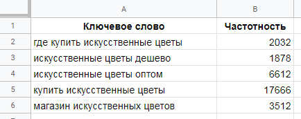
Example. There is a list of keys with frequencies. Our goal is to occupy the TOP-3. In this case, we want to choose only such keys, each of which will bring us at least 300 visitors per month.

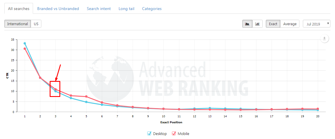
We determine how much traffic falls to the third position in the organic sector. To do this, go to this service and see that the third position results in about 10% of organic traffic (of course, this figure is inaccurate, but this is better than nothing).

We compose an IF expression that will return a value of 1 for the keys, which will result in a minimum of 300 visitors, and 0 for the remaining keys:

 =IF(B2*0.1>=300;"1";"0")
      
      

        
        
        
      

    
        
        
        
      
      

        
        
        
      

    
     

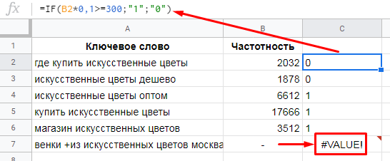
Please note that in line 7 the formula generated an error, since the frequency value was set in the wrong format. For such situations, there is an advanced version of the IF function - IFERROR.

Please note: the use of a comma or dot for decimal fractions in the formula is defined in the settings of your tables.

2. IFERROR - assign your value in case of an error

The function allows you to display the setpoint in a cell if an error is issued.

Syntax:

 =IFERROR( ;"   ")
      
      

        
        
        
      

    
        
        
        
      
      

        
        
        
      

    
     

We use this function in the example described above. Set the value in case of an error “no data”.

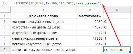
As you can see, the value is #VALUE! changed the view to understandable to us “no data”.

3. ARRAYFORMULA - stretch the formula down in one click

In working with data, almost every time you have to write down a formula for all cells in a column. “Pull” it by holding the left mouse button, or copy-paste - this is the last century.

It is enough to wrap the original function in the ARRAYFORMULA function, and the formula will apply to all the cells below. Moreover, if you delete adding rows, the formula will still work - without spaces in the calculations.

Syntax:

 =ARRAYFORMULA( )
      
      

        
        
        
      

    
        
        
        
      
      

        
        
        
      

    
     

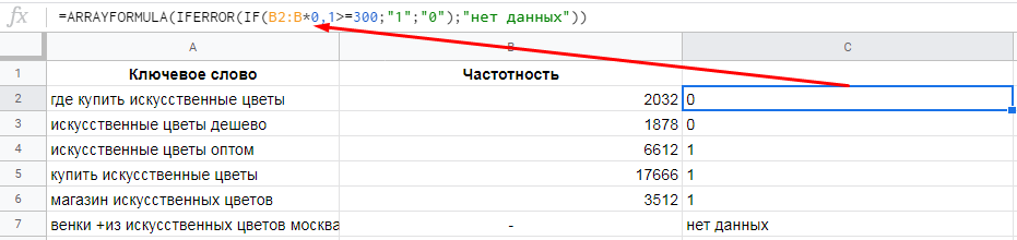
Example. We will automatically apply the formula described above for all cells in the range. To do this, we conclude the original formula in ARRAYFORMULA:

 =ARRAYFORMULA(IFERROR(IF(B2:B*0,1>=300;"1";"0");" "))
      
      

        
        
        
      

    
        
        
        
      
      

        
        
        
      

    
     

Please note that instead of cell B2 we specified the range for which we apply the formula (B2: B is the entire column B, starting from the second row). If you specify one cell, the formula will not work.

Life hack. Press CTRL + SHIFT + ENTER after entering the main formula, and the ARRAYFORMULA function will be applied automatically.

ARRAYFORMULA does not work with all functions. For example, it is not compatible with GOOGLETRANSLATE and IMPORTXML, which we will discuss below.

4. LEN - count the number of characters in the cell

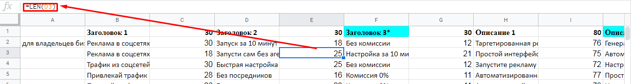
This feature is especially useful when composing contextual advertising ads - when it’s important not to overstep the allotted number of characters for headings, descriptions, display URLs, quick links and refinements.

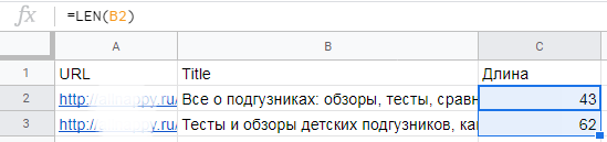
In SEO, the LEN function is used, for example, when composing title and description meta tags. Symbols function counts with spaces.

Syntax:

 =LEN(  )
      
      

        
        
        
      

    
        
        
        
      
      

        
        
        
      

    
     

Example. We need to make titles for all pages of the site. We know that about 55 characters are displayed in the search results. Our task is to compose titles so that the most important information is in the first 55 characters. We write the LEN formula for the filled cells. Now we know for sure when we approach the displayed 55 characters.

5. TRIM - remove spaces at the beginning and end of a phrase

When you parse semantics from different sources, it often contains “garbage” elements - spaces, pluses, special characters. Consider features that help quickly clean the core. One of them is TRIM.

This function removes spaces at the beginning and end of the phrase specified in the cell.

Syntax:

 =TRIM(,         )
      
      

        
        
        
      

    
        
        
        
      
      

        
        
        
      

    
     

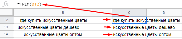
The function removes all spaces before and after the phrase - no matter how many there are.

6. SUBSTITUTE - change / delete spaces and special characters

Universal function to replace / delete characters in cells.

Syntax:

 =SUBSTITUTE( ;" ";"  "; )
      
      

        
        
        
      

    
        
        
        
      
      

        
        
        
      

    
     

Correspondence number - the serial number of the met value to replace, for example, replace the first met value, leave the rest. Optional parameter.

Example. We have an unloading of key phrases from Yandex.Wordstat. Many keys contain pluses. We need to remove them.

The formula will look like:

 =SUBSTITUTE(B12;"+";"";)
      
      

        
        
        
      

    
        
        
        
      
      

        
        
        
      

    
     

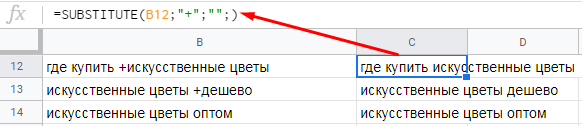
What have we done:

• where to search - indicated a cell with data;
• “What to look for” - indicated a plus sign that needs to be removed;
• “What to change for” - since the character needs to be deleted, we indicated quotation marks without characters inside; if we needed a replacement, here we would write the text for which we need to replace the plus sign;
• match number - here we did not specify anything, and the function will delete all the pluses in the phrase; if we specified 1, then the function would delete only the first plus sign, if 2 - the second, etc.

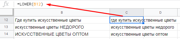
7. LOWER - translate letters from upper case to lower case

When compiling keys and parsing from different sources (for example, from competitors' meta tags), it may turn out that they will have upper case letters. To bring the keys in a unified form, you need to translate all the letters in lower case. To do this, use the LOWER function.

Syntax:

 =LOWER(,        )
      
      

        
        
        
      

    
        
        
        
      
      

        
        
        
      

    
     

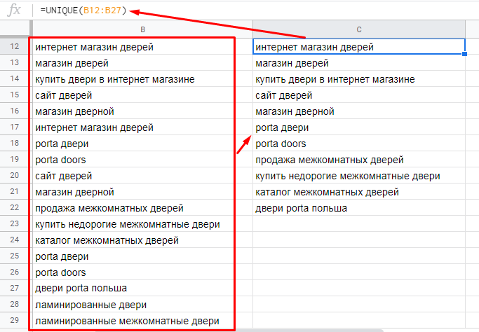
8. UNIQUE - output data without duplicate cells

The function analyzes the selected range for full takes and displays only unique lines - in the same order as in the original range.

Syntax:

 =UNIQUE( )
      
      

        
        
        
      

    
        
        
        
      
      

        
        
        
      

    
     

Example. We collected keys from Yandex.Wordstat, search tips, parsed the words of competitors. Naturally, in this array of keys we will have duplicates. We do not need them. We remove them using UNIQUE.

If you want to remove garbage from the kernel in one fell swoop, use the free word normalizer . It removes duplicate phrases (subject to permutations), changes the case, removes spaces and special characters. In essence, it does the same thing as the TRIM, SUBSTITUTE, LOWER, and UNIQUE functions combined - in just one click.

9. SEARCH - find the data in the line

With this function, you will quickly find the rows you need with a large amount of data.

Syntax:

 =SEARCH(« »; )
      
      

        
        
        
      

    
        
        
        
      
      

        
        
        
      

    
     

The function is used in different situations:

• highlight key phrases with the necessary intent (for example, branded or related to a specific topic, product or service);
• Find specific characters in the URL (for example, UTM parameters or a question mark)
• find URLs for link building purposes - for example, containing the words “guest-post”).

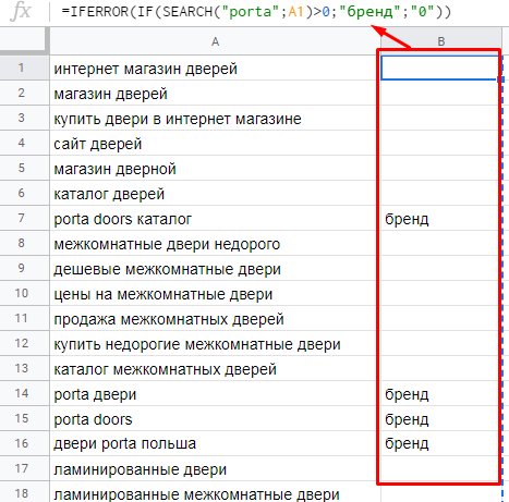
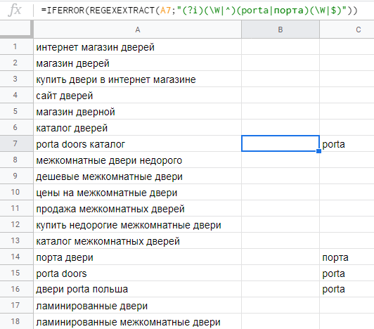
Example. We have a list of keys for the online door store. We want to find all branded queries and mark them in the table. To do this, use the formula:

 =SEARCH("porta";A1)
      
      

        
        
        
      

    
        
        
        
      
      

        
        
        
      

    
     

But in this form, the formula in the absence of the word "porta" in the key will show us #VALUE! .. In addition, if this word is in the desired cell, the function will put down the number of the character with which this word begins. The result looks like this:

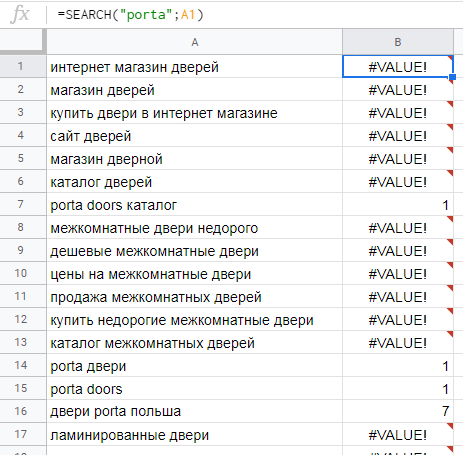
To obtain the search result in a form convenient for us, we additionally use the IF and IFERROR functions:

 =IFERROR(IF(SEARCH("porta";A1)>0;"";"0"))
      
      

        
        
        
      

    
        
        
        
      
      

        
        
        
      

    
     

10. SPLIT - break phrases into separate words

The function divides strings into fragments using the specified delimiter.

Syntax:

 =SPLIT(;"")
      
      

        
        
        
      

    
        
        
        
      
      

        
        
        
      

    
     

It should be borne in mind that the second half of the divided text will occupy the next column. So if you have a tight table, you need to add an empty column before applying the formula.

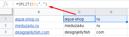
Example. We have a list of domains. We need to divide them into domain names and extensions. In the SPLIT function, specify a point as a separator and get the result:

11. CONCATENATE - combine data in cells

This function, unlike the previous one, combines data from several cells.

Syntax:

 =CONCATENATE( 1; 2;...)
      
      

        
        
        
      

    
        
        
        
      
      

        
        
        
      

    
     

Important: not only the values ​​of the cells, but also the characters (in quotation marks) can be inserted in the formula.

Example. In the example with the SPLIT function, we split the domains. Let's do the reverse operation using CONCATENATE (specify the cells to be merged and between them indicate the separator - period):

12. VLOOKUP - looking for values ​​in a different data range

The function searches for the key in the first column of the range and returns the value of the specified cell in the found row.

Syntax:

 =VLOOKUP(;;_;[])
      
      

        
        
        
      

    
        
        
        
      
      

        
        
        
      

    
     

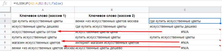
Example 1. There are two arrays of key phrases obtained from different sources. You need to find the keys in the first array that are not found in the second array. To do this, use the formula:

 =VLOOKUP(A2:A;B2:B;1;false)
      
      

        
        
        
      

    
        
        
        
      
      

        
        
        
      

    
     

What have we done:

• set the range A2: A, from which we take the keys for comparison;
• set the range B2: B, with which we compare the keys from column A;
• set the column number (1), from which we tighten the keys for matches;
• false - indicated that we do not need sorting.

The VLOOKUP function is often used when searching for data on different sheets or in different documents.

Example 2. We downloaded data from Yandex.Webmaster and Google Search Console about indexing pages on a site. Our task is to compare the data and determine which pages are indexed in one search engine, but not indexed in another.

We upload the results of the uploads to a Google Sheets file. On one sheet is the URL from Google, on the second from Yandex.

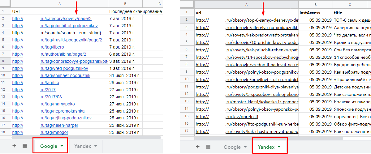
In cell C2, we write the VLOOKUP function. Immediately conclude in a function in ARRAYFORMULA to automatically pull down:

 =ARRAYFORMULA(VLOOKUP(A2:A;Yandex!A2:A;1;false))
      
      

        
        
        
      

    
        
        
        
      
      

        
        
        
      

    
     

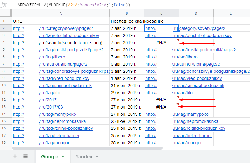
Now we immediately see which pages are indexed in Google, but not indexed in Yandex.

What have we done:

• set the range A2: A of the current sheet, from which we take the value for comparison;
• set the range Yandex! A2: A sheet with unloading from Yandex, with which we will compare the URL values ​​from Google;
• indicated the column number of the sheet with unloading from Yandex, the values ​​from which we pull up when the values ​​from the compared ranges coincide;
• false - indicated that we do not need sorting.

If you need to check the indexing of specific pages at the same time in Yandex and Google, use the tool from PromoPult. Download the list of URLs and run the check. If the page is indexed in a search engine, the column will have the number 1, if not - 0.

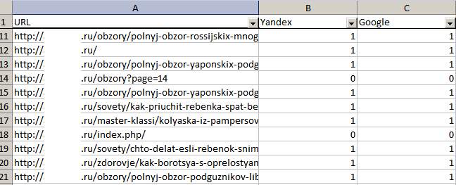
How to use this tool and in what situations it is useful, read in this guide .

13. IMPORTRANGE - import data from other tables

The function allows you to insert data from other tables into the current file.

Syntax:

 =IMPORTRANGE("  ";"   ")
      
      

        
        
        
      

    
        
        
        
      
      

        
        
        
      

    
     

Example:

 =IMPORTRANGE("https://docs.google.com/spreadsheets/d//"," !A2:A25")
      
      

        
        
        
      

    
        
        
        
      
      

        
        
        
      

    
     

Example. You are promoting a client’s site. Three specialists are working on the project: link builder, SEO specialist and copywriter. Everyone keeps a report. The client is interested in monitoring the process online. You create one report for it with tabs: “Links”, “Positions”, “Texts”. The IMPORTRANGE function pulls data on these tabs in each direction.

The advantage of the function is that you open access only to specific sheets. At the same time, the internal parts of expert reports remain inaccessible to customers.

14. IMPORTXML - parse data from web pages

Spreading function for parsing data from web pages using XPath.

Syntax:

 =IMPORTXML("url";"xpath-")
      
      

        
        
        
      

    
        
        
        
      
      

        
        
        
      

    
     

Here are just a few uses for this feature:

• extract metadata from the list of URLs (title, description), as well as h1-h6 headers;
• collecting e-mail from pages;
• parsing of page addresses in social networks.

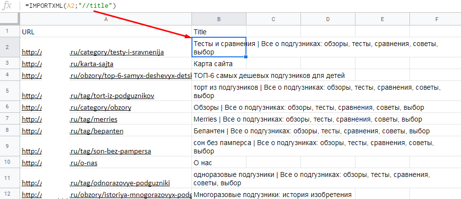
Example. We need to collect the contents of the title tags for the list of URLs. The XPath query that we use to get this header looks like this: "// title".

The formula would be:

 =IMPORTXML(A2;"//title")
      
      

        
        
        
      

    
        
        
        
      
      

        
        
        
      

    
     

IMPORTXML does not work with ARRAYFORMULA, so manually copy the formula to all cells.

Here are other XPath queries you might find useful:

• unload headers H1 (and by analogy - h2-h6): // h1
• parse meta tags description: // meta [@ name = 'description'] / @ content
• parse meta tags keywords: // meta [@ name = 'keywords'] / @ content
• extract e-mail addresses: // a [contains ( href , 'mailTo:') or contains ( href , 'mailto:')] / @ href
• extract links to profiles on social networks: // a [contains ( href , 'vk.com/') or contains ( href , 'twitter.com/') or contains ( href , 'facebook.com/') or contains ( href , 'instagram.com/') or contains ( href , 'youtube.com/'))/@href

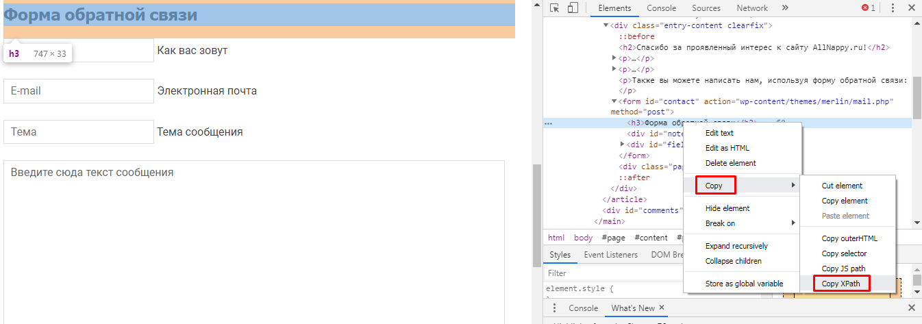
If you need to find out the XPath request for other elements of the page, open it in Google Chrome, go to the code view mode, find the element, right-click on it and click Copy / Copy XPath.

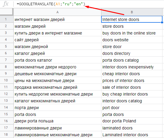
15. GOOGLETRANSLATE - translate keywords and other data

In multilingual projects, you often have to translate key phrases. This is most conveniently done using the GOOGLETRANSLATE function directly in the table.

Syntax:

 =GOOGLETRANSLATE(«»; [_]; [_])
      
      

        
        
        
      

    
        
        
        
      
      

        
        
        
      

    
     

For example, if we need to translate keys from Russian into English, the formula would be:

 =GOOGLETRANSLATE(A1;"ru";"en")
      
      

        
        
        
      

    
        
        
        
      
      

        
        
        
      

    
     

If we were translating from English into Russian, we would need to change the order of the languages:

 =GOOGLETRANSLATE(A1;"en";"ru")
      
      

        
        
        
      

    
        
        
        
      
      

        
        
        
      

    
     

GOOGLETRANSLATE does not work with ARRAYFORMULA, so, as in the case of IMPORTXML, we extend the formula manually.

16. REGEXEXTRACT - extract the desired text from the cells

This function allows you to extract text described by using RE2 regular expressions supported by Google from a data string. The syntax of regular expressions is quite complicated, you can find more examples in Google Help .

Syntax:

 =REGEXEXTRACT( ;” ”)
      
      

        
        
        
      

    
        
        
        
      
      

        
        
        
      

    
     

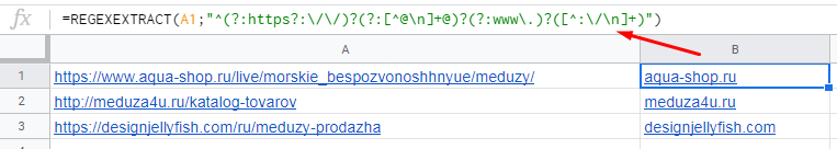
Example 1. We have a list of URLs. Need to extract domains. Here the regular expression will help us:

 ^(?:https?:\/\/)?(?:[^@\n]+@)?(?:www\.)?([^:\/\n]+)
      
      

        
        
        
      

    
        
        
        
      
      

        
        
        
      

    
     

Example 2. In the list of key phrases you need to find branded keys with the words "porta" and "port". To search for phrases containing any of these words, use the regular expression:

 (?i)(\W|^)(porta|)(\W|$)
      
      

        
        
        
      

    
        
        
        
      
      

        
        
        
      

    
     

As you can see, in the tables you can cut and cut the data as you need, just understand the formulas.