
The industrial development of software systems requires a lot of attention to the fault tolerance of the final product, as well as a quick response to failures and failures if they do happen. Monitoring, of course, helps to respond to failures and failures more efficiently and faster, but not enough. Firstly, it’s very difficult to keep track of a large number of servers - a large number of people are needed. Secondly, you need to understand how the application is designed to predict its state. Therefore, you need a lot of people who have a good understanding of the systems we are developing, their indicators and features. Suppose, even if you find a sufficient number of people who want to do this, it takes a lot of time to educate them.
What to do? Here, artificial intelligence hurries to our aid. This article will focus on predictive maintenance. This approach is actively gaining popularity. A large number of articles are written, including on Habré. Large companies are using this approach to support the performance of their servers. Having studied a large number of articles, we decided to try to apply this approach. What came of this?
Introduction
The developed software system sooner or later goes into operation. It is important for the user that the system works without failures. If an emergency situation does occur, it should be eliminated with minimal delay.
To simplify the technical support of a software system, especially if there are a lot of servers, monitoring programs are usually used that take metrics from a running software system, make it possible to diagnose its state and help determine what caused the failure. This process is called software system monitoring.
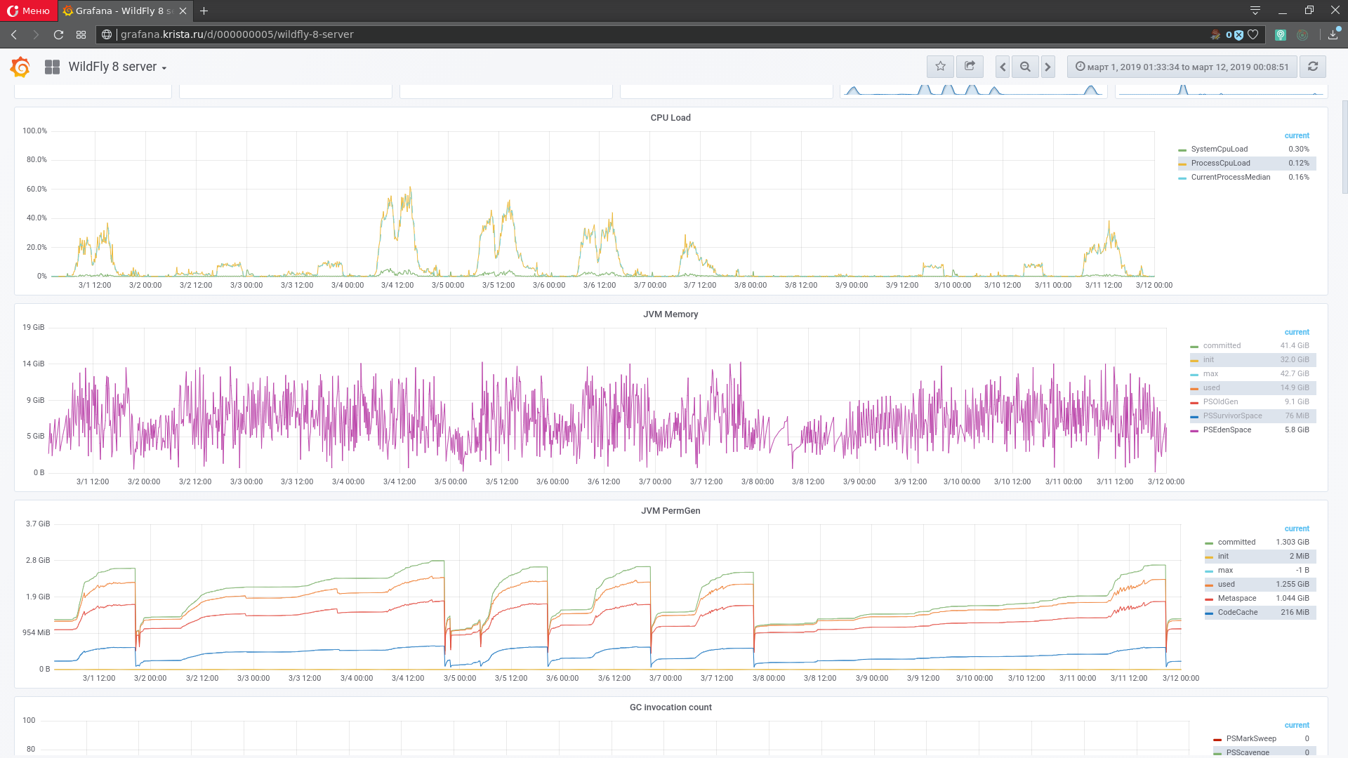
Figure 1. Interface for monitoring grafana
Metrics are various indicators of a software system, its execution environment, or a physical computer under which a system with a timestamp of the time that the metrics were received is running. In static analysis, metric data is called time series. To monitor the state of the software system, the metrics are displayed in the form of graphs: the time along the X axis and the values along the Y axis (Figure 1). Several thousand metrics (from each node) can be taken from a working software system. They form the space of metrics (multidimensional time series).
Since complex software systems take a large number of metrics, manual monitoring becomes a difficult task. To reduce the amount of data analyzed by the administrator, monitoring tools contain tools to automatically identify possible problems. For example, you can configure a trigger that works when the free disk space decreases to a specified threshold. You can also automatically diagnose a server shutdown or a critical slowdown in service speed. In practice, monitoring tools do a good job of detecting failures that have already occurred or identifying simple symptoms of future failures, but in general, predicting a possible failure remains a tough nut for them. Prediction by manual analysis of metrics requires the involvement of qualified specialists. It is unproductive. Most potential failures may go unnoticed.
Recently, the so-called predictive maintenance of software systems has become increasingly popular among large software development companies. The essence of this approach is to find problems leading to the degradation of the system in the early stages, before its failure using artificial intelligence. This approach does not exclude completely manual monitoring of the system. It is an aid to the monitoring process as a whole.
The main tool for implementing predictive maintenance is the task of searching for anomalies in time series, since when an anomaly occurs in the data, it is likely that after some time a malfunction or failure will occur . An anomaly is a certain deviation in the performance of a software system, such as detecting a degradation in the speed of a single request or a decrease in the average number of serviced calls at a constant level of client sessions.
The problem of finding anomalies for software systems has its own specifics. In theory, for each software system, it is necessary to develop or refine existing methods, since the search for anomalies very much depends on the data in which it is produced, and the data on software systems vary greatly depending on the system implementation tools up to which computer it is running under.
Anomaly search methods for predicting software system failures
First of all, it is worth saying that the idea of failure forecasting was inspired by the article “Machine Learning in IT Monitoring” . To test the effectiveness of the approach with automatic anomaly search, the Web-Consolidation software system was selected, which is one of the projects of the Krista NGO. For her, manual monitoring was previously performed according to the obtained metrics. Since the system is quite complex, a large number of metrics are taken for it: JVM indicators (garbage collector loading), OS indicators under which the code is executed (virtual memory,% CPU utilization os), network indicators (network load), server itself (CPU loading , memory), wildfly metrics and native application metrics for all critical subsystems.
All metrics are removed from the system using graphite. Initially, the whisper database was used as a standard solution for grafana, but with the growth of the client base, graphite ceased to cope, having exhausted the throughput of the disk subsystem of the DC. After that, it was decided to search for a more effective solution. The choice was made in favor of graphite + clickhouse , which allowed to reduce the load on the disk subsystem by an order of magnitude and reduce the occupied disk space by five to six times. Below is a diagram of the metrics collection mechanism using graphite + clickhouse (Figure 2).
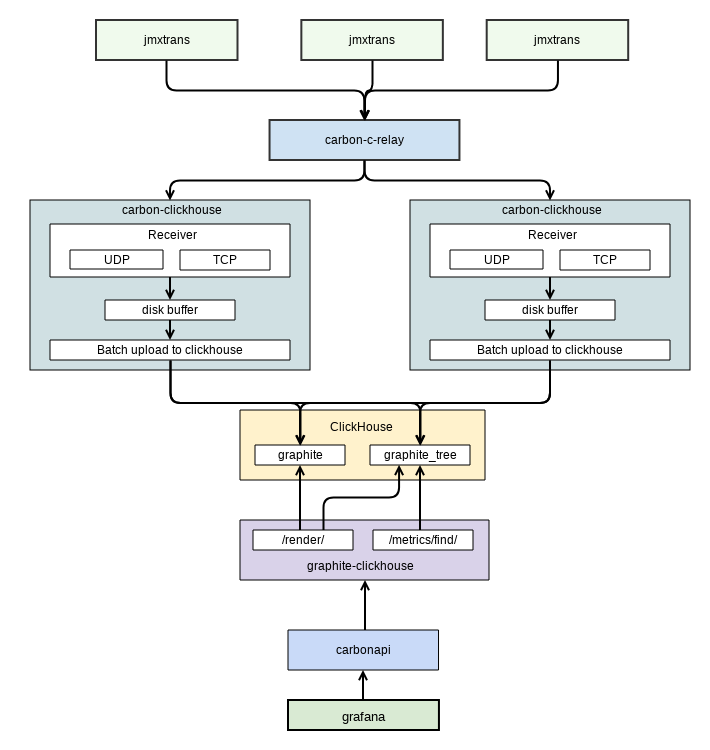
Figure 2. Metric removal chart
The diagram is taken from internal documentation. It shows the data exchange between grafana (the user interface for monitoring that we use) and graphite. Removing metrics from the application produces a separate software - jmxtrans . He adds them to graphite.
The Web Consolidation system has a number of features that create problems for predicting failures:
- a trend change often occurs. Various versions are available for this software system. Each of them carries changes in the software part of the system. Accordingly, in this way, developers directly affect the metrics of this system and can cause a change in trend;
- the implementation peculiarity, as well as the purpose of using this system by customers, often cause anomalies without previous degradation;
- the percentage of anomalies relative to the entire data set is small (<5%);
- there may be gaps in the receipt of indicators from the system. At some short intervals, the monitoring system fails to obtain metrics. For example, if the server is overloaded. This is critical for training a neural network. There is a need to fill in the gaps synthetically;
- Cases with anomalies are often relevant only for a specific date / month / time (seasonality). This system has clear rules for use by its users. Accordingly, metrics are relevant only for a specific time. The system may not be used constantly, but only in some months: selectively depending on the year. There are situations when the same behavior of metrics in one case can lead to a software system failure, but not in another.
To begin with, methods for detecting anomalies in the monitoring data of software systems were analyzed. In articles on this subject, with small percentages of anomalies relative to the rest of the data set, neural networks are most often proposed.
The basic logic for searching for anomalies using data from neural networks is shown in Figure 3:

Figure 3. Search for anomalies using a neural network
Based on the forecast or recovery of the window of the current flow of metrics, the deviation from that obtained from a working software system is calculated. In the case of a big difference between the received metrics from the software system and the neural network, we can conclude that the current data length is anomalous. The following series of problems arise for the use of neural networks:
- for correct operation in streaming mode, the data for training models of neural networks should include only “normal” data;
- You must have an up-to-date model for correct detection. A change in trend and seasonality in metrics can cause a large number of false positives for the model. To update it, it is necessary to clearly define the time when the model is obsolete. If you update the model later or earlier, then most likely a large number of false positives will follow.
Also, one should not forget about the search and prevention of the frequent occurrence of false positives. It is assumed that they will most often occur in emergency situations. However, they can also be a consequence of a neural network error due to insufficient training. It is necessary to minimize the number of false positives of the model. Otherwise, false forecasts will spend a lot of time for the administrator who is intended to check the system. Sooner or later, the administrator will simply stop responding to the “paranoid” monitoring system.
Recurrent neural network
To detect anomalies in the time series, a recurrent neural network with LSTM memory can be used. The only problem is that it can only be used for predicted time series. In our case, not all metrics are predictable. An attempt to apply RNN LSTM for a time series is shown in Figure 4.
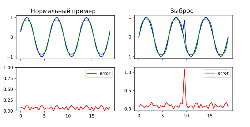
Figure 4. An example of a recurrent neural network with LSTM memory cells
As can be seen from Figure 4, the RNN LSTM managed to cope with the search for anomalies in this time section. Where the result has a high forecast error (mean error), an anomaly in terms of indicators actually occurred. Using one RNN LSTM will obviously not be enough, because it is applicable to a small number of metrics. It can be used as an auxiliary method of searching for anomalies.
Failure prediction auto encoder
An auto - encoder is essentially an artificial neural network. The input layer is encoder, the output layer is decoder. The disadvantage of all neural networks of this type is that it poorly localizes anomalies. The synchronous auto-encoder architecture was chosen.
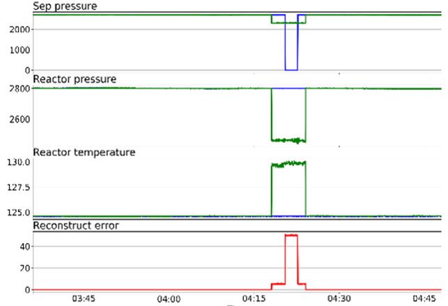
Figure 5. Example auto-encoder operation
Autocoders learn from normal data and then find something abnormal in the data supplied to the model. Just what you need for this task. It remains only to choose which of the auto-encoders is suitable for this task. The architecturally simplest form of autocoding is a direct, irreversible neural network, which is very similar to a multilayer perceptron (MLP), with an input level, output level and one or more hidden layers connecting them.
However, the differences between auto-encoders and MLP are that in an automatic encoder, the output level has the same number of nodes as the input, and that instead of learning to predict the target value Y given by input X, the auto-encoder learns to reconstruct its own X. Therefore Auto-encoders are uncontrolled training models.
The task of the auto-encoder is to find the temporal indices r0 ... rn corresponding to the anomalous elements in the input vector X. This effect is achieved by searching for the quadratic error.

Figure 6. Synchronous Auto Encoder
A synchronous architecture was chosen for the auto-encoder. Its advantages: the ability to use streaming processing mode and a relatively smaller number of neural network parameters relative to other architectures.
False positive minimization mechanism
Due to the fact that various emergency situations arise, as well as a situation of insufficient training of the neural network, a decision was made about the need to develop a mechanism for minimizing false positives for the developed model for detecting anomalies. This mechanism is based on a template base that the administrator classifies.
The dynamic timeline transformation algorithm (DTW-algorithm, from the English. Dynamic time warping) allows you to find the optimal match between time sequences. First used in speech recognition: used to determine how two speech signals represent the same original spoken phrase. Subsequently, application was found for him in other areas.
The basic principle of minimizing false positives is to collect a reference database using an operator that classifies suspicious cases detected using neural networks. Next, the classified standard is compared with the case that the system detected, and it is concluded that the case belongs to a false or leading to failure. Just for comparison of two time series the DTW algorithm is also used. The main tool for minimization is still classification. It is assumed that after collecting a large number of reference cases, the system will begin to ask the operator less because of the similarity of most cases and the occurrence of similar ones.
As a result, on the basis of the above-described methods of neural networks, an experimental program was built to predict the failures of the Web-Consolidation system. The purpose of this program was to use the existing archive of monitoring data and information about failures that had already occurred to evaluate the competence of this approach for our software systems. The scheme of the program is presented below, in figure 7.
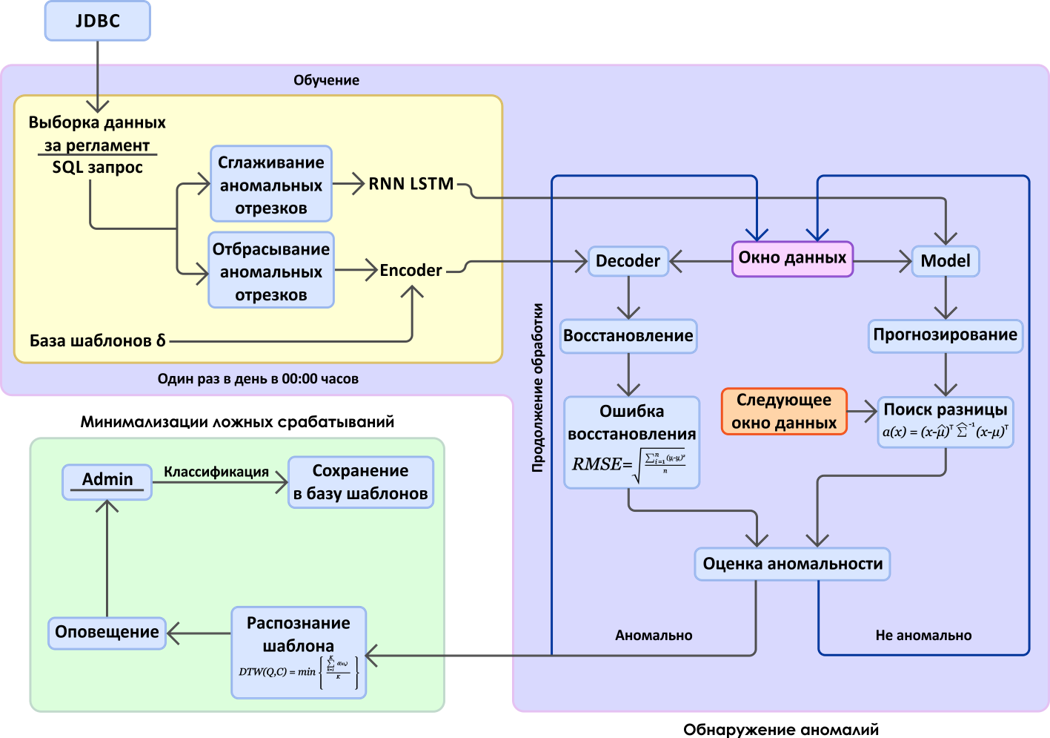
Figure 7. Failure prediction diagram based on metric space analysis
Two main blocks can be distinguished in the diagram: the search for abnormal time periods in the monitoring data stream (metrics) and the mechanism for minimizing false positives. Note: for experimental purposes, data is obtained through a JDBC connection from the database into which graphite will save it.
The following is the interface obtained as a result of the development of a monitoring system (Figure 8).
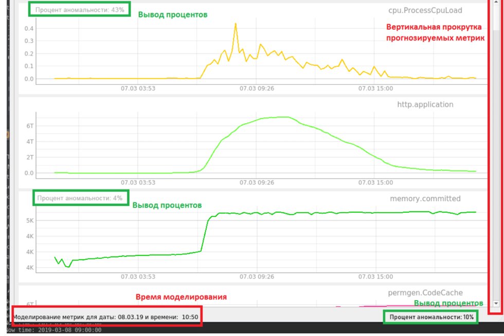
Figure 8. The interface of the experimental monitoring system
The percentage of anomalousness in the received metrics is displayed on the interface. In our case, the receipt is modeled. We already have all the data for several weeks and ship them gradually to verify the case of an anomaly leading to failure. The lower status bar displays the total percentage of data anomalies at a given time, which is determined using an auto-encoder. Also, for forecasted metrics, a separate percentage is displayed that calculates the RNN LSTM.
An example of detecting anomalies in CPU performance using the RNN LSTM neural network (Figure 9).

Figure 9. RNN LSTM discovery
A fairly simple case, essentially a normal outlier, but leading to a system failure, was successfully calculated using the RNN LSTM. The anomaly indicator in this time interval is 85 - 95%, everything above 80% (the threshold is determined experimentally) is considered an anomaly.
An example of anomaly detection when the system could not boot after the update. This situation is detected by the auto-encoder (Figure 10).
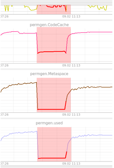
Figure 10. Example auto-encoder detection
As can be seen from the figure, PermGen hovered at the same level. The auto-encoder found this strange because he had not seen anything like it before. Here the anomaly holds all 100% until the system returns to a healthy state. Anomaly is displayed across all metrics. As mentioned earlier, an auto-encoder cannot localize anomalies. The operator is called upon to perform this function in these situations.
Conclusion
PC "Web-Consolidation" is developed not the first year. The system is in a fairly stable state, and the number of recorded incidents is small. Nevertheless, it was possible to find anomalies leading to failure 5 to 10 minutes before the failure. In some cases, a notification of a failure in advance would help save the scheduled time that is allocated for carrying out “repair” work.
For those experiments that have been carried out, it is too early to draw final conclusions. At the moment, the results are contradictory. On the one hand, it is clear that algorithms based on neural networks are able to find “useful” anomalies. On the other hand, a large percentage of false positives remains, and not all anomalies detected by a qualified specialist in the neural network can be detected. The disadvantages include the fact that now the neural network requires training with a teacher for normal work.
For the further development of the system for predicting failures and bringing it to a satisfactory state, several ways can be envisaged. This is a more detailed analysis of cases with anomalies that lead to failure, due to this addition to the list of important metrics that greatly affect the state of the system, and the rejection of unnecessary ones that do not affect it. Also, if we move in this direction, we can try to specialize the algorithms specifically for our cases with anomalies that lead to failures. There is another way. This is an improvement in the architecture of neural networks and an increase in detection accuracy due to this reduction in training time.
I express my gratitude to the colleagues who helped me with writing and supporting the relevance of this article: Viktor Verbitsky and Sergey Finogenov.