
In America, it is very difficult to live without a car, and since we sold our cars before moving, now we had to buy a new family vehicle. I decided to approach the solution of this problem as any good specialist in data processing and analysis would approach. I decided to use the data.
Data collection
Often the most difficult part of a data research project is the data collection phase. Especially when it comes to some kind of home project. It is very likely that downloading from the Internet something ready for processing, formatted as a CSV file, will fail. And without data, neither a model nor a forecast can be built.
How to get data on the car market? Web scraping will help us solve this problem.

Google Chrome Developer Tools
Web scraping is an automated process of collecting data from websites. I am not an expert in web scraping, and this article is not a guide to collecting data from sites. But, if you practice a little and delve into the features of some Python modules, you can satisfy the craziest fantasies regarding data collection.
In this project, I used the Selenium Python package, which is a browser without a user interface. Such a browser opens pages and works with them in the same way a user would work with them (unlike something like the Beautiful Soup Python library, which simply reads HTML code).
Thanks to the tools of the Google Chrome developer, the process of preparing for data collection is greatly simplified. It all comes down to right-clicking on the elements of web pages that interest us and copying them to
xpath
,
element_id
, or anything else. All this is well perceived by Selenium. But sometimes you have to tinker a bit to find the element and text you need.
The code I used to collect information on hundreds of cars can be found here .
Data cleansing
One of the problems with data collected through web scraping is that this data is very likely to be pretty untidy. The point here is that they were not taken from a certain repository, but collected from a website that was created in order to show information to people. As a result, such data needs serious cleaning. Often this means that you need to parse strings to get the data you need.
After I saved the web scraping results to a CSV file, I was able to load this data into the Pandas data frame and do the cleaning.
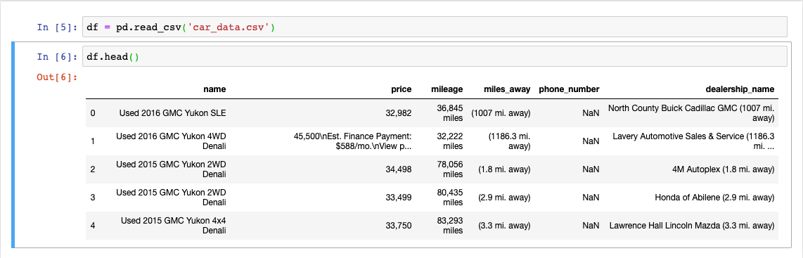
Data before cleaning
Now I could, using something like regular expressions, start extracting the information I needed from the collected data, and create features that I could investigate, and based on which I could build models.
First I created a regex function suitable for reuse that I could pass to the Pandas
.apply
method.
def get_regex_item(name, pattern): item = re.search(pattern, name) if item is None: return None else: return item.group()
The
name
column has a lot of useful data. Based on it, using the function I created, I could create four new features.
df['4wd'] = df.name.apply(lambda x: 1 if get_regex_item(x, pattern= r'4[a-zA-Z]{2}') else 0) df['year'] = df.name.apply(lambda x: get_regex_item(x, pattern= r'\d{4}')) df['type'] = df.name.apply(lambda x: x.split()[-1]) df['certified'] = df.name.apply(lambda x: 1 if get_regex_item(x.lower(), r'certified') else 0) df['price'] = df.price.apply(lambda x: x[:6].replace(",", "")).astype('int') df['mileage'] = df.mileage.apply(lambda x: x.split()[0].replace(",", "")).astype('int')
As a result, I got the data frame shown in the following figure.
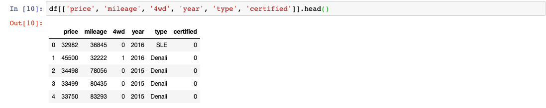
Data after cleaning
Exploratory data analysis
Now it's time to do something interesting. Namely, exploratory data analysis. This is a very important step in the work of a data scientist, since it allows you to understand the features of the data, see the trends and interactions. My target variable was price, as a result, I built graphical representations of the data, focusing on the price.
import matplotlib.pyplot as plt import seaborn as sns plt.gca().spines['top'].set_visible(False) plt.gca().spines['right'].set_visible(False) #box plots sns.boxplot(x = df.year, y=df.price, data=df[['year', 'price']], color='purple') sns.boxplot(x = df.type, y=df.price, data=df[['year', 'price']], color='cyan')
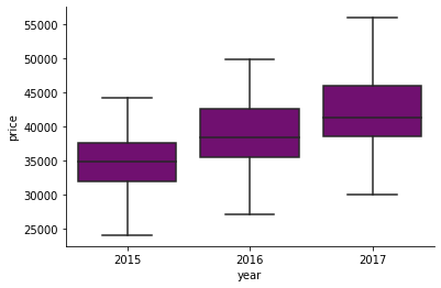
The dependence of the price of the car on the year of its release
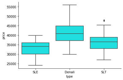
The dependence of the price on the type of car
These box charts, reflecting the relationship between price and some categorical variables, give very clear signals that the price is highly dependent on the year of manufacture and on the type of car.
And here is the scatter chart.
import matplotlib.pyplot as plt import seaborn as sns plt.gca().spines['top'].set_visible(False) plt.gca().spines['right'].set_visible(False) #scatter plot sns.regplot(x=df.mileage, y=df.price , color='grey')

Scatter chart
Here, analyzing the dependence of price on mileage, I again saw a strong correlation between the independent variable (
mileage
) and the price of the car. There is a strong negative relationship, since as the mileage of the car increases, its price drops. Given what everyone knows about cars, this is understandable.
Knowing the relationship between some of the independent variables and the target variable, we can get a pretty good idea of what features are especially important and what type of model to use.
Independent Character Encoding
Another step that had to be done before building the model was to code independent features. Signs
4wd
and
certified
already presented in a logical form. They do not need additional processing. But the signs of
type
and
year
need to be encoded. To solve this problem, I used the Pandas
.get_dummies
method, which allows encoding with one active state.
Pandas is a fairly intelligent system that allowed me to pass all the attributes to it and encoded only independent variables, and also allowed me to remove one of the columns just created in order to get rid of the attributes that are completely correlated with each other. The use of such data would lead to errors in the model and in its interpretation. Please note that in the end I only had two columns with information about the year of manufacture of the machine, since column
_2015
was deleted. The same goes for
type
columns.
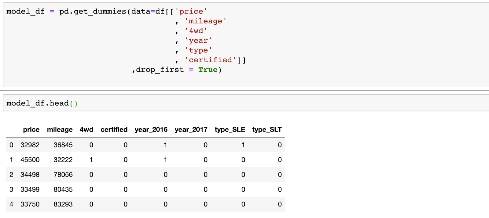
Data After Encoding Independent Variables
Now my data turned out to be converted into a format on the basis of which I could build a model.
Model creation
Based on the analysis of the above diagrams, and on what I know about cars, I decided that in my case a linear model would do.
I used the OLS linear regression model (Ordinary Least Squares, the usual least squares method). To build the model, the statsmodel Python package was used.
import statsmodels.api as sm y = model_df.price X = model_df.drop(columns='price') model = sm.OLS(y, X).fit() print(model.summary())
Here are the simulation results.
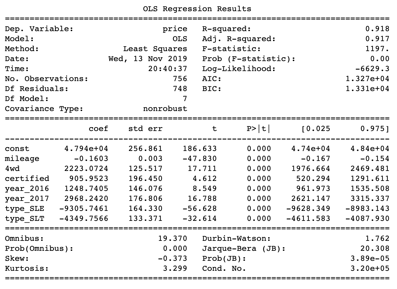
Simulation resulted in a standard error of 1556.09
The obtained coefficients correspond to what could be seen in the diagrams during the exploratory data analysis. Mileage has a negative effect on price. On average, every extra thousand miles you drive leads to a price reduction of $ 1,600. This is true for GMC Yukon cars, perhaps not for everyone. Probably the most shocking results of all were those that point to the price difference between SLE (low-end Yukon cars) and Denali (high-end Yukon cars). The difference is over $ 9000. This means that a buyer of a higher class car has to pay a lot of money for all the premium options he receives. As a result, it would be nice if he really needed all this.
What kind of car is it worth buying?
So, I collected, cleaned, parsed, researched, visualized the data and built a model based on them. But the original question of what to buy after all remained unanswered. How to find out that a certain offer is worth accepting?
The approach to finding the answer to this question is very simple. You need to use the model to form a forecast and find the difference between the predicted price and the price that car dealers offer. Then you need to sort the list of price differences so that the most undervalued offers are at the top of it. This will give a list of the most advantageous offers.
After taking into account some additional restrictions (my budget and my wife’s preferences), I was able to get on a sorted list of offers and started phoning sellers.
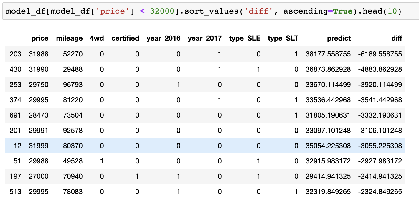
The car we bought is highlighted in blue
In the end, we bought the 2015 GMC Yukon Denali for $ 32,000. It was $ 3000 cheaper than the forecast issued by the model.
Although there were more advantageous offers on the market, the car we bought was not far from us, which greatly simplified and accelerated the purchase process. Given that at that time we did not have a car, speed and convenience in solving this issue were important to us.
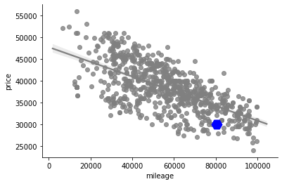
Our purchase is highlighted in blue on the diagram
In the end, we were able to look at one of the previously compiled diagrams, displaying on it information about the purchased car. This showed us that we, indeed, found a good option.
My wife really likes her new car, but I like the price of this car. In general, summing up the above, we can say that we bought the car successfully.
Dear readers! Do you use data analysis tools to solve any everyday problems?