“I think I can safely say that no one understands quantum mechanics,” Richard Feynman
The subject of quantum computing has always attracted technical writers and journalists. Her computational potential and complexity gave her a kind of mystical halo. Too often thematic articles and infographics describe in detail all kinds of prospects for this industry, while barely touching on the issues of its practical application: this may mislead a not-too-careful reader.
In popular science articles, descriptions of quantum systems are omitted and statements like:
A regular bit can be equal to "1" or "0", but a qubit can be simultaneously equal to "1" and "0".
If you are very lucky (of which I am not sure), then they will tell you that:
The qubit is in a superposition between “1” and “0”.
None of these explanations seems plausible, because we are trying to formulate a quantum-mechanical phenomenon using language tools created in a very traditional world. To clearly explain the principles of quantum computing, it is necessary to use another language - mathematical.
In this guide, I will talk about the mathematical tools needed to model and understand quantum computing systems, as well as how to illustrate and apply the logic of quantum computing. Moreover, I will give an example of a quantum algorithm and tell what is its advantage over a traditional computer.
I will do my best to talk about all this in an understandable language, but still I hope that the readers of this article have basic ideas about linear algebra and digital logic (linear algebra is described here , digital logic is here ).
To get started, let's go over the principles of digital logic. It is based on the use of electrical circuits for calculations. To make our description more abstract, we simplify the state of the wire to “1” or “0”, which will correspond to the “on” or “off” states. Having built transistors in a certain sequence, we will create the so-called logic elements that take one or more values of the input signals and convert them into an output signal based on certain rules of Boolean logic.
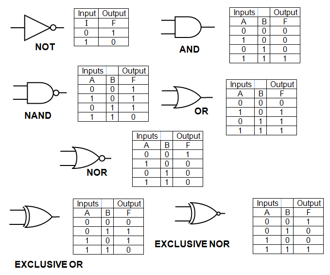
Common logic elements and state tables
Based on the chains of such basic elements, you can create more complex elements, and on the basis of chains of more complex elements we can ultimately rely on obtaining an analogue of the central processor with a high degree of abstractness.
As I mentioned earlier, we need a way to mathematically map digital logic. To get started, let's introduce the traditional mathematical logic. Using linear algebra, classic bits with the values “1” and “0” can be represented as two column vectors:
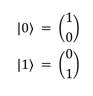
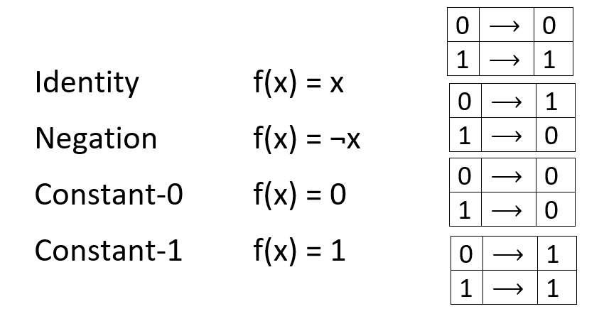
where the numbers on the left are the Dirac vector notation . By representing our bits in this way, we can model logical operations on bits using vector transformations. Please note: despite the fact that when using two bits in logic elements, you can perform many operations (“AND” (AND), “Not” (NOT), “Exclude Or” (XOR), etc.), when using one bits it is possible to perform only four operations: the identity conversion, negation, calculation of the constant "0" and the calculation of the constant "1". During the identical conversion, the bit remains unchanged, when negated, the bit value is reversed (from “0” to “1” or from “1” to “0”), and the calculation of the constant “1” or “0” sets the bit to “1” or "0" regardless of its previous value.
| Identity
| Identity transformation
|
| Negation
| Negation
|
| Constant-0
| Calculation of the constant "0"
|
| Constant-1
| Calculation of the constant "1"
|
Based on our new representation of a bit, it is quite easy to perform operations on the corresponding bit using vector transformation:

Before moving on, let's look at the concept of reversible computing , which only implies that in order to ensure the reversibility of an operation or logical element, it is necessary to determine a list of input signal values based on the output signals and the names of the operations used. Thus, we can conclude that the identity transformation and negation are reversible, but the operation of calculating the constants “1” and “0” is not. Due to the unitarity of quantum mechanics, quantum computers use exclusively reversible operations, which is why we will focus on them. Next, we will convert irreversible elements to reversible ones in order to ensure the possibility of their use by a quantum computer.
Using the tensor product of individual bits, many bits can be represented:

Now that we have almost all the necessary mathematical concepts, we will move on to our first quantum logic element. This is the CNOT operator, or the controlled "NOT" (NOT), which is of great importance in reversible and quantum computing. The CNOT element is applied to two bits and returns two bits. The first bit is assigned as “control”, and the second - “control”. If the control bit is set to “1”, the control bit changes its value; if the control bit is set to “0”, the control bit does not change.
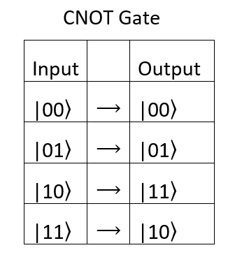
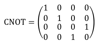
This operator can be represented as the following transformation vector:
To demonstrate everything that we have already dealt with, I will show you how to use the CNOT element with respect to many bits:
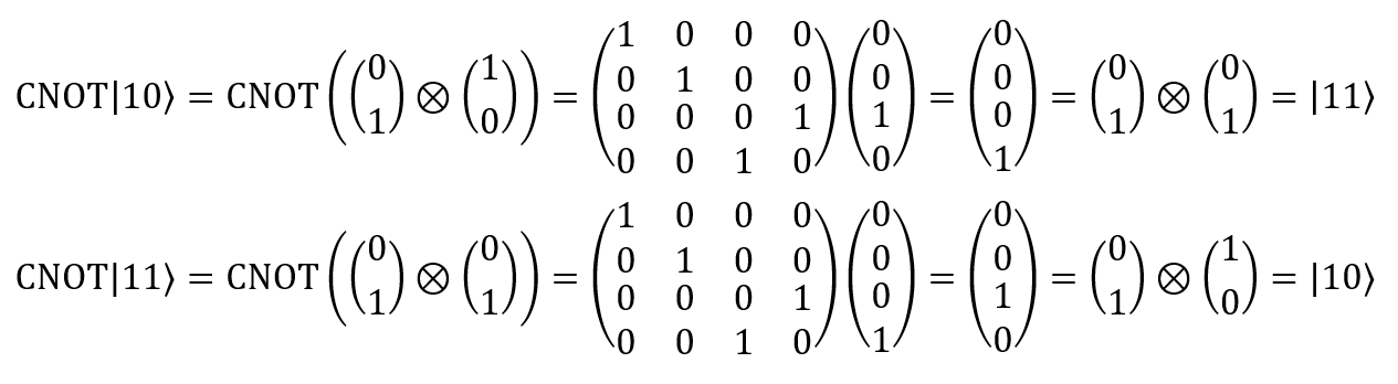
We summarize what has already been said: in the first example we decompose | 10⟩ into parts of its tensor product and use the CNOT matrix to obtain a new corresponding state of the product; then we factor it to | 11⟩ according to the table of CNOT values given earlier.
So, we remembered all the mathematical rules that will help us deal with traditional calculations and ordinary bits, and finally we can move on to modern quantum computing and qubits.
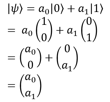
If you read up to this place, then I have good news for you: qubits can easily be expressed mathematically. In general, if the classic bit (cbit) can be set to | 1⟩ or | 0⟩, the qubit is simply in superposition and can be equal to | 0⟩ and | 1⟩ before measurement. After measurement, it collapses at | 0⟩ or | 1⟩. In other words, a qubit can be represented as a linear combination of | 0⟩ and | 1⟩ in accordance with the formula below:
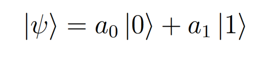
where a₀ and a₁ represent, respectively, the amplitudes | 0⟩ and | 1⟩. They can be considered as “quantum probabilities”, which represent the probability of a qubit collapsing into any of the states after its measurement, since in quantum mechanics an object in superposition collapses into one of the states after fixing. Expand this expression and get the following:
In order to simplify my explanation, I will use this notion in this article.
For this qubit, the chance of collapsing to a₀ after measurement is | a ₀ | ², and the chance of collapse into a ₁ is | a ₁ | ². For example, for the following qubit:

the chance of collapse in "1" is | 1 / √2 | ², or ½, that is, 50/50.
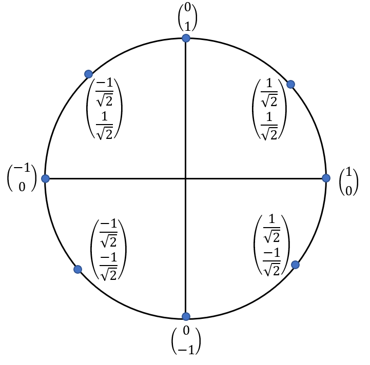
Since in the classical system all the probabilities in the sum must give unity (for a full probability distribution), we can conclude that the squares of the absolute values of the amplitudes | 0⟩ and | 1⟩ must total one. Based on this information, we can compose the following equation:

If you are familiar with trigonometry, you will notice that this equation corresponds to the Pythagorean theorem (a² + b² = c²), that is, we can graphically represent the possible states of the qubit in the form of points on the unit circle, namely:
Logical operators and elements are applied to qubits as well as in the case of classical bits - based on matrix transformation. All reversible matrix operators that we have recalled up to now, in particular, CNOT, can be used to work with qubits. Such matrix operators make it possible to use each of the amplitudes of a qubit without measuring and collapsing it. Let me give you an example of using the negation operator to qubit:

Before we continue, I recall that the amplitudes a ₀ and a ₁ are actually complex numbers , so the qubit state can most accurately be displayed on a three-dimensional unit sphere, also known as the Bloch sphere :

However, to simplify the explanation, here we restrict ourselves to real numbers.
It seems that the time has come to discuss some of the logical elements that make sense exclusively in the context of quantum computing.
One of the most important operators is the “Hadamard element”: it takes a bit in the “0” or “1” state and puts it in the corresponding superposition with a 50% chance of collapsing it to “1” or “0” after the measurement.
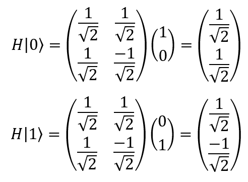
Note that there is a negative number in the lower right side of the Hadamard operator. This is due to the fact that the result of applying the operator depends on the value of the input signal: - | 1⟩ or | 0⟩, and therefore the calculation is reversible.
Another important point related to the Hadamard element is its reversibility, that is, it can take a qubit in the corresponding superposition and convert it to | 0⟩ or | 1⟩.

This is very important because it allows us to transform from a quantum state without determining the state of the qubit - and, accordingly, without collapsing it. So, we can structure quantum computing on the basis of a deterministic rather than a probabilistic principle.
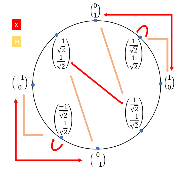
Quantum operators containing exclusively real numbers are their own opposite, so we can present the result of applying the operator to a qubit as a transformation within the unit circle in the form of a state machine:

Thus, the qubit, whose state is shown in the diagram above, after applying the Hadamard operation is converted to the state indicated by the corresponding arrow. Similarly, we can construct another state machine that will illustrate the transformation of a qubit using the negation operator, as shown above (also known as the Pauli negation operator, or bit inversion), as shown below:

To perform more complex operations with our qubit, you can use a chain of many operators or apply elements many times. An example of a serial transformation based on the representation of a quantum chain is as follows:

That is, if we start with the bit | 0⟩, apply the bit inversion, and then the Hadamard operation, then another bit inversion, and again the Hadamard operation, after which the final bit inversion, we get the vector on the right side of the chain. By superimposing various state machines on top of each other, we can start with | 0⟩ and track the colored arrows corresponding to each of the transformations in order to understand how this all works.
Since we have gone this far, it's time to consider one of the types of quantum algorithms, namely the Deutsch-Joji algorithm , and show its advantage over a classical computer. It is worth noting that the Deutsch-Joji algorithm is completely deterministic, that is, it returns the correct answer in 100% of cases (unlike many other quantum algorithms based on the probabilistic determination of qubits).
Let's imagine that you have a black box that contains a function / operator on one bit (remember - when using one bit, only four operations are possible: identically transform, negate, calculate the constant “0” and calculate the constant “1”). What function is performed in a box? You do not know which one, however, you can sort out as many variants of input values as you like and evaluate the results at the output.
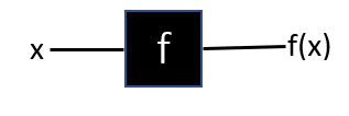
How many input and output signals will have to be driven through the black box to find out which function is used? Think about it for a second.
In the case of a classic computer, you will need to make 2 queries to determine the function used. For example, if when entering “1” we get “0” at the output, it becomes clear that either the function for calculating the constant “0” or the negation function is used, after which you will have to change the value of the input signal to “0” and see what happens at the exit.
In the case of a quantum computer, you will also need two queries, since you still need two different output values to determine the exact function that applies to the input value. However, if we reformulate the question a bit, it turns out that quantum computers still have a serious advantage: if you wanted to find out if the function used is constant or variable, the superiority would be on the side of quantum computers.
The function used in the box is a variable, if different values of the input signal give different results on the output (for example, the identical conversion and inversion of the bit), and if the output value does not change regardless of the input value, then the function is constant (for example, calculating the constant “1” or the calculation of the constant “0”).
Using the quantum algorithm, you can determine if a function in a black box is constant or variable based on just one request. But before we examine in detail how to do this, we need to find a way that will allow us to structure each of these functions on a quantum computer. Since any quantum operators must be invertible, we immediately encounter a problem: the functions for calculating the constants "1" and "0" are not.
In quantum computing, the following solution is often used: an additional output qubit is added, which returns any value of the input signal received by the function.
| Before:
| After:
|

| 
|
Applying the same representation of the quantum chain that we used earlier, we will see how each of the four elements (identity transformation, negation, calculation of the constant “0” and calculation of the constant “1”) can be implemented using quantum operators.
For example, this way you can implement the function of calculating the constant "0":
Calculation of the constant "0":
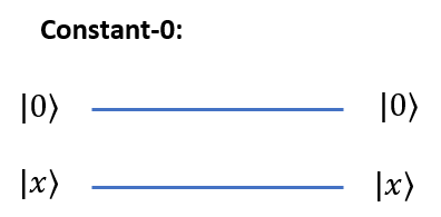
Here we do not need operators at all. The first input qubit (which we took equal to | 0⟩) returns with the same value, and the second input value returns itself - as usual.
With the function for calculating the constant “1”, the situation is slightly different:
Calculation of the constant "1":

Since we accepted that the first input qubit is always set to | 0⟩, as a result of applying the bit inversion operator, it always gives one at the output. And as usual, the second qubit gives its own value at the output.
When the identity transformation operator is displayed, the task begins to become more complicated. Here's how to do it:
Identity Transformation:

The symbol used here denotes the CNOT element: the upper line indicates the control bit, and the lower line indicates the control bit. Let me remind you that when using the CNOT operator, the value of the control bit changes if the control bit is | 1⟩, but remains unchanged if the control bit is | 0⟩. Since we assumed that the value of the upper line is always equal to | 0⟩, its value is always assigned to the lower line.
Similarly, we act with the negation operator:
Negation:
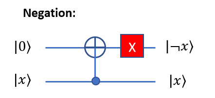
We simply invert the bit at the end of the output line.
Now that we’ve figured out the preliminary presentation, let's look at the specific advantages of a quantum computer over a traditional computer when it comes to determining the constancy or variability of a function hidden in a black box using only one query.
To solve this problem using quantum computing in a single query, it is necessary to translate the input qubits into a superposition before they are transferred to the function, as shown below:

The Hadamard element is reapplied to the result of using the function to derive qubits from the superposition and make the algorithm deterministic. We start the system in the state | 00⟩ and for the reasons that I will talk about now, we get the result | 11⟩ if the function used is constant. If the function inside the black box is variable, then after measuring the system returns the result | 01⟩.
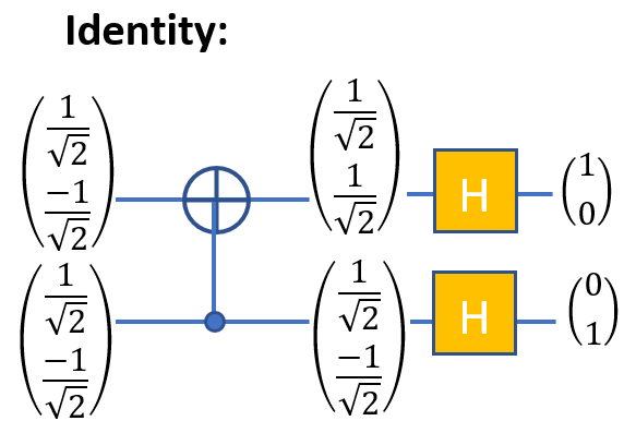
To deal with the rest of the article, let's turn to the illustration I showed earlier:
Using the bit inversion operator, and then applying the Hadamard element to both input values equal to | 0⟩, we will ensure their translation into the same superposition | 0⟩ and | 1⟩, namely:

Using the example of transferring this value to a function in a black box, it is easy to demonstrate that both functions of a constant value give | 11⟩ to the output.
Calculation of the constant "0":
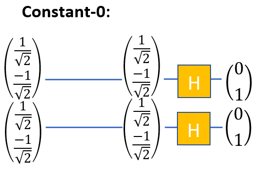
Similarly, we see that the function for calculating the constant “1” also gives | 11⟩, that is:
Calculation of the constant "1":

Please note: at the output, both values will be equal to | 1⟩, since -1² = 1.
Using the same principle, we can prove that when using both variable functions, we will always get | 01 (if the same method is used), although here everything is a little more complicated.
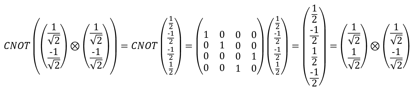
Identity Transformation:
Since CNOT is a two-qubit operator, it cannot be represented as a simple state machine, and therefore it is necessary to determine two output signals based on the tensor product of both input qubits and multiplication by the CNOT matrix according to the previously described principle:
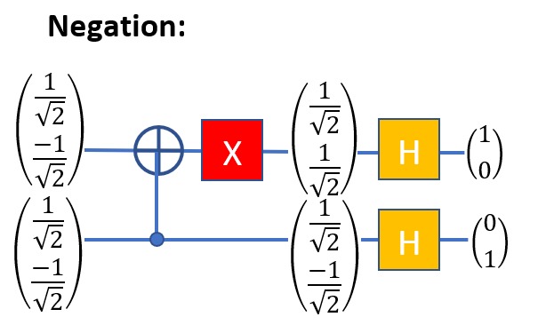
Using this method, we can also confirm that the output has the value | 01 if the negation function is hidden in the black box:
Negation:
Thus, we have just demonstrated a situation in which a quantum computer is uniquely more efficient than a conventional computer.
What next?
I propose to end this. We did a great job already. If you understand everything that I talked about, I think that now you are well versed in the basics of quantum computing and quantum logic, and also understand why in certain situations quantum algorithms can be more effective than traditional means of calculation.
It is difficult to call my description a complete guide to quantum computing and algorithms - it is rather a brief introduction to mathematics and the notation system, designed to dispel the reader’s ideas about the subject imposed by popular science sources (seriously, many really can not figure out the situation!). I did not have time to touch on many important topics — for example, such as the quantum entanglement of qubits , the complex nature of the amplitudes | 0⟩ and | 1⟩, and the functioning of various quantum logic elements during transformation by the Bloch sphere.
If you want to systematize and structure your knowledge of quantum computers, I highly recommend that you read Emma Strubel's An Introduction to Quantum Algorithms : Despite the abundance of mathematical formulas, this book discusses quantum algorithms in much more detail.