We study the statement of the central limit theorem using the exponential distribution

Instead of introducing

The article describes a study conducted to verify the statement of the central limit theorem that the sum of N independent and identically distributed random variables selected from almost any distribution has a distribution close to normal. However, before we proceed to the description of the study and a more detailed disclosure of the meaning of the central limit theorem, it will not be out of place to tell why the study was conducted at all and to whom the article may be useful.



First of all, the article can be useful for all beginners to understand the basics of machine learning, especially if a respected reader is also in his first year of specialization “Machine Learning and Data Analysis”. It is this kind of research that needs to be carried out in the final week of the first course, the above specialization, in order to receive the coveted certificate.

Research approach

So, back to the question of research. What the central limit theorem tells us. But she says this. If there is a random value X from practically any distribution, and a sample of volume N is randomly generated from this distribution, then the sample average determined on the basis of the sample can be approximated by a normal distribution with an average value that coincides with the mathematical expectation of the original population.



For the experiment, we need to choose a distribution from which a sample will be randomly generated. In our case, we will use the exponential distribution.



So, we know that the probability density of the exponential distribution of a random variable X has the form:

$$ $$ display $$ f (x) = \ lambda \ varepsilon ^ {- \ lambda x} $$ display $$

where $$ $ inline $ x> 0 $ inline $ , $$ $ inline $ \ lambda> 0 $ inline $



The mathematical expectation of a random variable X , in accordance with the law of exponential distribution is determined, inversely $$ $ inline $ \ lambda $ inline $ : $$ $ inline $ \ mu = \ frac {1} {\ lambda} $ inline $



The variance of a random variable X is defined as $$ $ inline $ \ sigma ^ 2 = \ frac {1} {\ lambda ^ 2} $ inline $



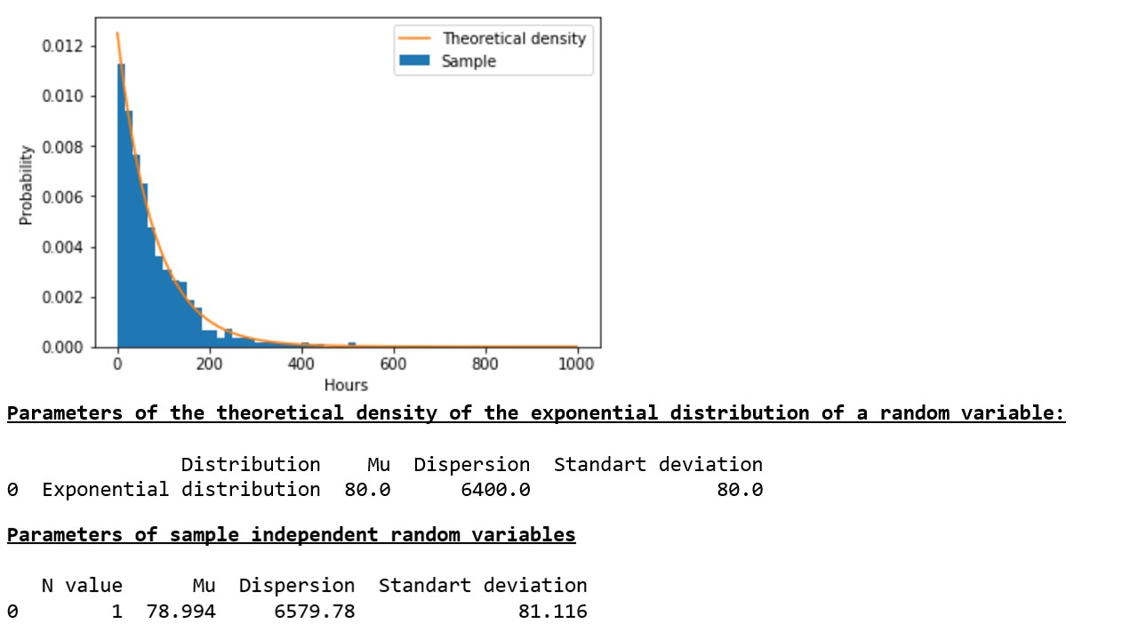
Our study uses the exponential distribution parameter $$ $ inline $ \ lambda = 0.0125 $ inline $ then $$ $ inline $ \ mu = 80 $ inline $ , $$ $ inline $ \ sigma ^ 2 = 6400 $ inline $



To simplify the perception of values ​​and the experiment itself, suppose that we are talking about the operation of the device with an average expectation of uptime of 80 hours. Then, the more time the device will work, the less likely that there will be no failure and vice versa - when the device tends to zero time (hours, minutes, seconds), the probability of its failure also tends to zero.



Now from the exponential distribution with the given parameter $$ $ inline $ \ lambda = 0.0125 $ inline $ let's choose 1000 pseudo-random values. Compare the results of the sample with the theoretical probability density.



Further, and this is the most important thing in our small study, we will form the following samples. We take 3, 15, 50, 100, 150, 300, and 500 random variables from the exponential distribution, determine for each volume (from 3 to 500) the arithmetic mean, and repeat 1000 times. For each sample, we construct a histogram and superimpose on it a graph of the density of the corresponding normal distribution. We estimate the resulting parameters of the sample mean, variance, and standard deviation.



This could complete the article, but there is a proposal to somewhat expand the boundaries of the experiment. Let us estimate how much these parameters, with an increase in the sample size from 3 to 500, will differ from their counterparts - the same parameters of the corresponding normal distributions. In other words, we are invited to answer the question: will we observe a decrease in deviations with an increase in the sample size?



So, on the way. Our tools today will be the Python language and the Jupyter notebook.

We study the statement of the central limit theorem

The source code of the study is posted on the github

Attention! This file requires a Jupyter notebook!



A sample of a pseudo-random value generated by us in accordance with the law of exponential distribution 1000 times quite well characterizes the theoretical (initial) population (graph 1 *, table 1).



Chart 1, Table 1







Now let's see what happens if we take not just one pseudo-random value 1000 times, but the arithmetic average of 3, 15, 50, 100, 150, 300, or 500 pseudo-random values ​​and compare the parameters of each sample with the parameters of the corresponding normal distributions (graph 2 ** , table 2).



Chart 2



























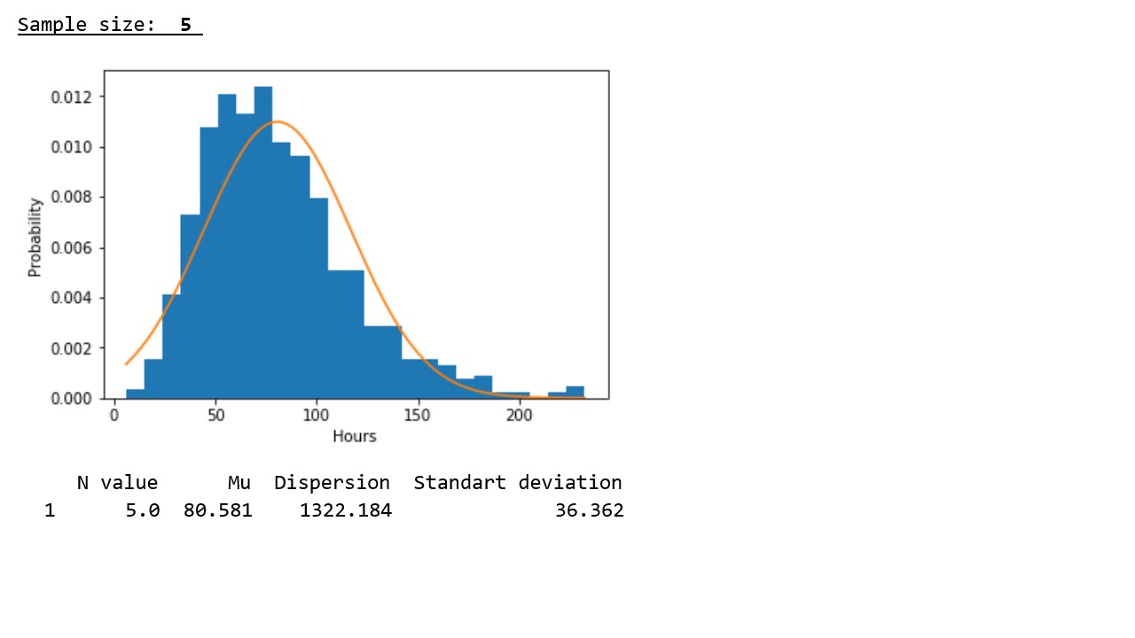
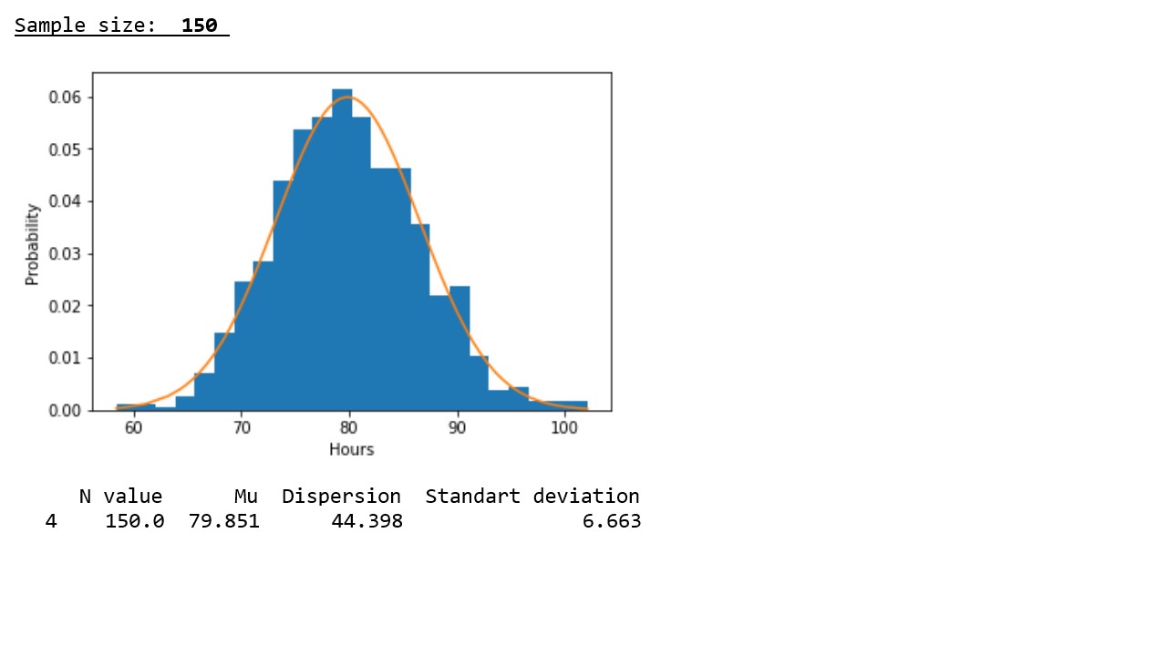
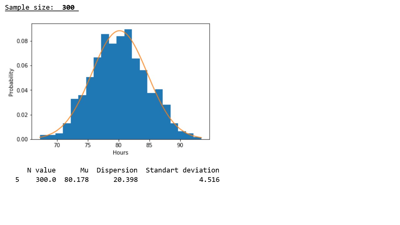
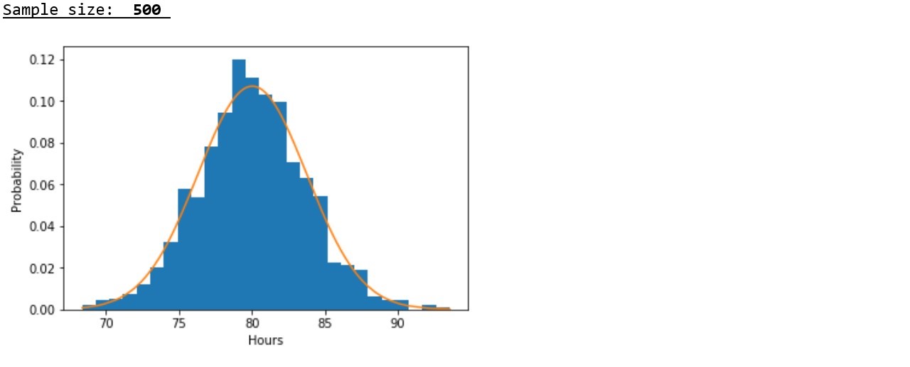
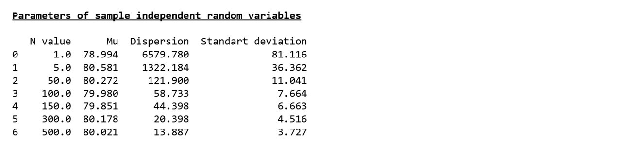
table 2







In accordance with the graphical representation of the results, the following regularity is clearly seen: with increasing sample size, the distribution approaches normal and the concentration of pseudorandom variables around the sample mean occurs, and the sample mean approaches the mathematical expectation of the initial distribution.



In accordance with the data presented in the table, the regularity revealed in the graphs is confirmed - with an increase in the sample size, the variances and standard deviations noticeably decrease, which indicates a denser concentration of pseudorandom values ​​around sample averages.



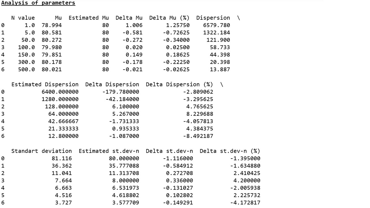
But that's not all. We remember that at the beginning of the article, a proposal was made to check whether, with increasing sample size, the deviations of the sample parameters with respect to the parameters of the corresponding normal distribution decrease.



As you can see (graph 3, table 3), an arbitrarily noticeable reduction in deviations does not occur - the parameters of the samples jump to plus or minus at different distances and do not want to stably approach the calculated values. We will try to find an explanation for the lack of positive dynamics in the following studies.



Chart 3







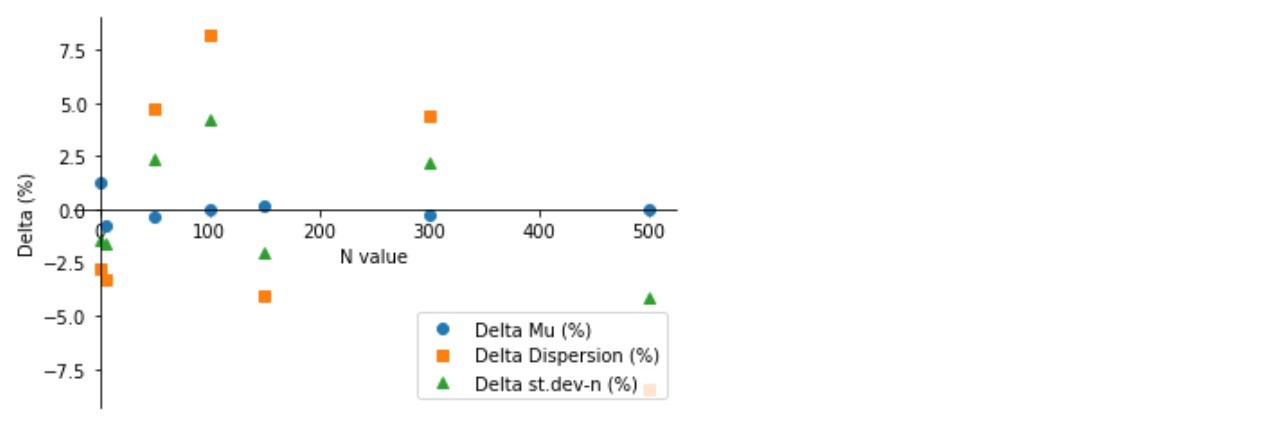
Table 3

Instead of conclusions

Our study, on the one hand, once again, confirmed the conclusions of the central limit theorem on the approximation of independent randomly distributed values ​​to the normal distribution with increasing sample size, on the other hand, it was possible to successfully complete the training of the first year of great specialization.



* Developing the logic of the example with equipment, the uptime of which is 80 hours, along the “X” axis we designate the clock - the less time it works, the less the probability of failure.



** A different interpretation of the X-axis values ​​is required here - the probability that the device will work at about 80 hours is the highest and, accordingly, it decreases as with an increase in operating time (that is, it is unlikely that the device will work much longer than 80 hours) , and with a decrease in operating time (the likelihood that the device will fail in less than 80 hours is also small).