What the Moscow metro would look like in a three-dimensional world
UPD: As requested in the comments, I add a link to the Javascript revolving schema
Unfortunately, javascript code could not be inserted into the body of the post
Good afternoon! Recently I read a blog by an urbanist who was discussing what an ideal metro scheme should be like. The metro scheme can be drawn based on two principles:
Obviously, these principles are mutually exclusive and the first principle requires a significant distortion of geographical reality.
It is enough to recall what the Moscow metro scheme looks like with beautiful rings and straight lines:
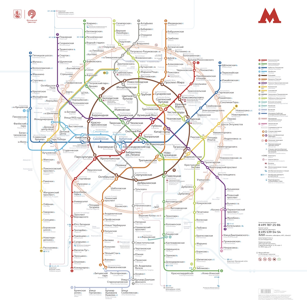
and compare with a geographically accurate plan:

It can be seen on the plan that the rings are not at all perfectly smooth and concentric, the lines bend much more than in the scheme, and the density of stations in the city center is so high that it is almost impossible to figure out the plan.
And although the second image reflects reality much more accurately, it can be seen that it is more convenient to use the first scheme for planning a route in the metro.
And then the following thought came to my mind: “What would the metro look like if the criterion for constructing the circuit were the time required to move from one station to another?” That is, if you can get from one station to another quickly, then spatially they would be located nearby on the diagram.
Obviously, in two-dimensional space it is impossible to draw such a scheme in which the distance between two stations would equal the travel time from one to the other due to the complex topology of the metro graph.
There is also a hunch that this is exactly possible when constructing a scheme in a space with a high dimension (the upper estimate is n-1, where n is the number of stations). For a space with a small number of dimensions, such a scheme can only be constructed approximately.
The task of constructing a metro map by travel time looks like a typical optimization task.
Suppose we have an initial set of coordinates of all stations (X, Y, Z) and a target matrix of pairwise times (distances). It is possible to construct the “incorrectness” metric of a given set of coordinates and then minimize it by the gradient descent method for each of the coordinates of each station. As a metric, we can take a simple function of the standard deviation of the distances.
Well, the only thing left is to get data on how much time should be spent on traveling from any station of the Moscow metro to any other.
The first thought was to check the Yandex metro api and get this data out of there. Unfortunately, the api description could not be found. Watch the times manually in the application for a long time (there are 268 stations in the metro and the time matrix size is 268 * 268 = 71824). Therefore, I decided to understand the source data of Yandex Metro. Since there is no access to the server, an apk file with the application was downloaded and the necessary data was found. All information about the metro is remarkably structured and stored in JSON format in the assets / metrokit / apk archive folder of the application. All data is stored in self-explanotary structures. Meta.json contains information about the cities whose schemes are present in the application, as well as the id of these schemes.
By the id of the scheme, we find the folder with JSON related to Moscow.
The data.json file contains basic information about the metro graph, including the names of the nodes of the graph, node IDs, geographical coordinates of nodes, information about transitions from one station to another (id, time of transition, type of transition - whether driving or walking, on the street or not, time We are interested in seconds) and also a lot of additional information about the entrances and exits from the station. This is easy enough to figure out. Let's start writing code to build our circuit.
We import the necessary libraries:
The structure of python dictionaries and lists is fully consistent with the structure of the json format, so we read the metro information and create objects that correspond to json objects.
We create a dictionary that maps the nodes of the graph and the station (this is necessary because the stations are assigned to the names, not the nodes of the graph)
Also, just in case, we will save the coordinates of the nodes for the possibility of constructing a geographical map (normalized to a range of 0-1)
Create a metro graph with connections. We set the weights of each connection. Weight corresponds to travel time. We will remove nodes that are not stations (in my opinion, these are exits from the metro and the connections to them are needed for Yandex cards when calculating the time, but did not understand it exactly), create a node id dictionary, the real name in Russian
We define which branch (which branch id) each node belongs to (this will be needed later for coloring metro lines in the diagram)
the networkx library allows you to find the shortest path length from one node to another using the nx.shortest_path_length (G, id1, id2, weight = 'length') function, so we can assume that we’ve finished the data preparation. The next thing to do is prepare a model that will optimize the coordinates of the stations.
To do this, we will figure out what will be given to the input, to the output, and how we will optimize the station coordinate matrix.
Suppose we have a matrix of all coordinates (3x268). Multiplication of one-hot vector (a vector where 0 is everywhere except one unit coordinate in place of n) of dimension 268 by this coordinate matrix will give 3 coordinates corresponding to station n. If we take a pair of one-hot vectors and multiply them by the required matrix, we get two triples of coordinates. From a pair of coordinates, you can calculate the Euclidean distance between stations. Thus, we can determine the architecture of our model:
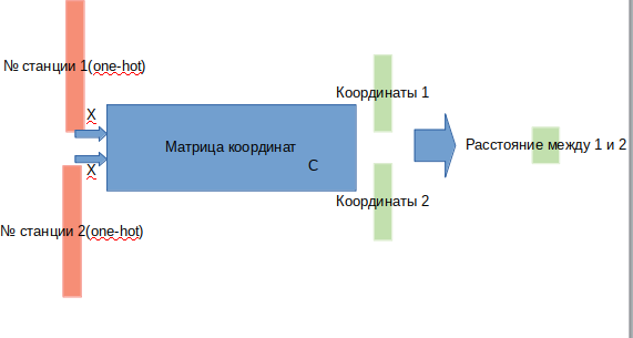
at the entrance we give a couple of stations, at the output we get the distance between them.
After we have decided on the data format for training the model, we will prepare the data using the distance search on the graph:
We optimize the matrix of station coordinates using the gradient descent method.
If we use the keras framework for machine learning, we get the following:
note that we use real geographical coordinates as the initial coordinates in layer1 — this is necessary in order not to fall into the local minimum of the standard deviation function. We initialize the third coordinate to non-zero to obtain a non-zero gradient (if at the beginning the map is absolutely flat, the shift of any station up or down will be the same, therefore the gradient is 0 and z will not be optimized). The last element of our model (Dense (1)) affects the scaling of the scheme to fit the timeline.
We will measure the distance in hours, not seconds, since the orders of distances are about 1 hour, and for more effective training of the model it is important that all values (input data, weights, targets) are approximately the same order of magnitude. If these values are close to 1, then you can use the standard step values for optimization (0.001-0.01).
The line model.layers [2] .trainable = False freezes the coordinates of the stations and at the first stage one parameter varies - the scale. After selecting the scale of our scheme, we unfreeze the coordinates and optimize them already:
we see that we feed all pairs of stations at once, at the exit all distances and our optimization is full batch gradient descent (one step on all data). The loss function in this case is the standard deviation and it can be seen that it was 0.015 at the end of training, which means the standard deviation of less than 1 minute for any pair of stations. In other words, the resulting scheme allows you to accurately know the distance that is required to get from one station to another by the distance in a straight line between stations with an accuracy of + -1 minute!
But let's see what our circuit looks like!
get the coordinates of the stations, take the color coding of the lines and build a 3d image with signatures (the code for a beautiful display of signatures is taken from here ):
Since there were difficulties with converting to an interactive 3d format for the browser, I post the gifs:
the version without text looks more beautiful and recognizable:
UPD: Add metro lines of the desired color and create a gif. Black lines - transitions between stations:
From this scheme, some interesting conclusions can be drawn that are not so obvious from other schemes. For some branches, for example, green, blue or violet, the MCC (pink ring) is practically useless due to uncomfortable transplants, which can be seen in the distance of the ring from these branches. The longest routes are from a communal apartment to a snapping or Pyatnitsky highway (red and pink / blue horses); long routes are also Alma-Ata storytelling and Bunin Alley-Nekrasovka. Judging by the plan, in the north of Moscow there is a partial duplication of gray and light green branches - they are nearby in the diagram. It would be interesting to see how the new lines (WDC, BKL) and who will use them more often. In any case, I hope such schemes can be interesting tools for analysis, inspiration and travel planning.
PS 3D is not necessary, for the 2D version it is enough to slightly correct the code. But in the case of the 2d scheme, it is impossible to achieve such accuracy of distances.
Unfortunately, javascript code could not be inserted into the body of the post
Good afternoon! Recently I read a blog by an urbanist who was discussing what an ideal metro scheme should be like. The metro scheme can be drawn based on two principles:
- The circuit should be convenient and easy to remember and orient.
- The scheme should correspond to the geography of the city
Obviously, these principles are mutually exclusive and the first principle requires a significant distortion of geographical reality.
It is enough to recall what the Moscow metro scheme looks like with beautiful rings and straight lines:
and compare with a geographically accurate plan:
It can be seen on the plan that the rings are not at all perfectly smooth and concentric, the lines bend much more than in the scheme, and the density of stations in the city center is so high that it is almost impossible to figure out the plan.
And although the second image reflects reality much more accurately, it can be seen that it is more convenient to use the first scheme for planning a route in the metro.
And then the following thought came to my mind: “What would the metro look like if the criterion for constructing the circuit were the time required to move from one station to another?” That is, if you can get from one station to another quickly, then spatially they would be located nearby on the diagram.
Obviously, in two-dimensional space it is impossible to draw such a scheme in which the distance between two stations would equal the travel time from one to the other due to the complex topology of the metro graph.
There is also a hunch that this is exactly possible when constructing a scheme in a space with a high dimension (the upper estimate is n-1, where n is the number of stations). For a space with a small number of dimensions, such a scheme can only be constructed approximately.
The task of constructing a metro map by travel time looks like a typical optimization task.
Suppose we have an initial set of coordinates of all stations (X, Y, Z) and a target matrix of pairwise times (distances). It is possible to construct the “incorrectness” metric of a given set of coordinates and then minimize it by the gradient descent method for each of the coordinates of each station. As a metric, we can take a simple function of the standard deviation of the distances.
Well, the only thing left is to get data on how much time should be spent on traveling from any station of the Moscow metro to any other.
The first thought was to check the Yandex metro api and get this data out of there. Unfortunately, the api description could not be found. Watch the times manually in the application for a long time (there are 268 stations in the metro and the time matrix size is 268 * 268 = 71824). Therefore, I decided to understand the source data of Yandex Metro. Since there is no access to the server, an apk file with the application was downloaded and the necessary data was found. All information about the metro is remarkably structured and stored in JSON format in the assets / metrokit / apk archive folder of the application. All data is stored in self-explanotary structures. Meta.json contains information about the cities whose schemes are present in the application, as well as the id of these schemes.
{ "id": "sc77792237", "name": { "en": "Nizhny Novgorod", "ru": " ", "tr": "Nizhny Novgorod", "uk": "і " }, "size": { "packed": 30300, "unpacked": 145408 }, "tags": [ "published" ], "aliases": [ "nizhny-novgorod" ], "logoUrl": "https://avatars.mds.yandex.net/get-bunker/135516/f2f0e33d8def90c56c189cfb57a8e6403b5a441c/orig", "version": "2c27fe1", "geoRegion": { "delta": { "lat": 0.168291, "lon": 0.219727 }, "center": { "lat": 56.326635, "lon": 43.992153 } }, "countryCode": "RU", "defaultAlias": "nizhny-novgorod" }
By the id of the scheme, we find the folder with JSON related to Moscow.
The data.json file contains basic information about the metro graph, including the names of the nodes of the graph, node IDs, geographical coordinates of nodes, information about transitions from one station to another (id, time of transition, type of transition - whether driving or walking, on the street or not, time We are interested in seconds) and also a lot of additional information about the entrances and exits from the station. This is easy enough to figure out. Let's start writing code to build our circuit.
We import the necessary libraries:
import numpy as np import json import codecs import networkx as nx import matplotlib.pyplot as plt import pandas as pd import itertools import keras import keras.backend as K from mpl_toolkits.mplot3d import Axes3D from mpl_toolkits.mplot3d.proj3d import proj_transform from matplotlib.text import Annotation import pickle
The structure of python dictionaries and lists is fully consistent with the structure of the json format, so we read the metro information and create objects that correspond to json objects.
names = json.loads(codecs.open( "l10n.json", "r", "utf_8_sig" ).read() ) graph = json.loads(codecs.open( "data.json", "r", "utf_8_sig" ).read() )
We create a dictionary that maps the nodes of the graph and the station (this is necessary because the stations are assigned to the names, not the nodes of the graph)
Also, just in case, we will save the coordinates of the nodes for the possibility of constructing a geographical map (normalized to a range of 0-1)
nodeStdict={} for stop in graph['stops']['items']: nodeStdict[stop['nodeId']]=stop['stationId'] coordDict={} for node in graph['nodes']['items']: coordDict[node['id']]=(node['attributes']['geoPoint']['lon'],node['attributes']['geoPoint']['lat']) lats=[] longs=[] for value in coordDict.values(): lats.append(value[1]) longs.append(value[0]) for k,v in coordDict.items(): coordDict[k]=((v[0]-np.min(longs))/(np.max(longs)-np.min(longs)),(v[1]-np.min(lats))/(np.max(lats)-np.min(lats)))
Create a metro graph with connections. We set the weights of each connection. Weight corresponds to travel time. We will remove nodes that are not stations (in my opinion, these are exits from the metro and the connections to them are needed for Yandex cards when calculating the time, but did not understand it exactly), create a node id dictionary, the real name in Russian
G=nx.Graph() for node in graph['nodes']['items']: G.add_node(node['id']) #graph['links'] for link in graph['links']['items']: #G.add_edges_from([(link['fromNodeId'],link['toNodeId'])]) G.add_edge(link['fromNodeId'], link['toNodeId'], length=link['attributes']['time']) nodestoremove=[] for node in G.nodes(): if len(G.edges(node))<2: nodestoremove.append(node) for node in nodestoremove: G.remove_node(node) labels={} for node in G.nodes(): try: labels[node]=names['keysets']['generated'][nodeStdict[node]+'-name']['ru'] except: labels[node]='error'
We define which branch (which branch id) each node belongs to (this will be needed later for coloring metro lines in the diagram)
def getlines(graph, G): nodetoline={} id_from={} id_to={} for lk in graph['tracks']['items']: id_from[lk['id']]=lk['fromNodeId'] id_to[lk['id']]=lk['toNodeId'] for line in graph['linesToTracks']['items']: if line['trackId'] in id_from.keys(): nodetoline[id_from[line['trackId']]]=line['lineId'] nodetoline[id_to[line['trackId']]]=line['lineId'] return nodetoline lines=getlines(graph,G)
the networkx library allows you to find the shortest path length from one node to another using the nx.shortest_path_length (G, id1, id2, weight = 'length') function, so we can assume that we’ve finished the data preparation. The next thing to do is prepare a model that will optimize the coordinates of the stations.
To do this, we will figure out what will be given to the input, to the output, and how we will optimize the station coordinate matrix.
Suppose we have a matrix of all coordinates (3x268). Multiplication of one-hot vector (a vector where 0 is everywhere except one unit coordinate in place of n) of dimension 268 by this coordinate matrix will give 3 coordinates corresponding to station n. If we take a pair of one-hot vectors and multiply them by the required matrix, we get two triples of coordinates. From a pair of coordinates, you can calculate the Euclidean distance between stations. Thus, we can determine the architecture of our model:
at the entrance we give a couple of stations, at the output we get the distance between them.
After we have decided on the data format for training the model, we will prepare the data using the distance search on the graph:
myIDs=list(G.nodes()) listofinputs1=[] listofinputs2=[] listofoutputs=[] for pair in itertools.product(G.nodes(), repeat=2): vec1=np.zeros((len(myIDs))) vec2=np.zeros((len(myIDs))) vec1[myIDs.index(pair[0])]=1 vec2[myIDs.index(pair[1])]=1 listofinputs1.append(vec1) listofinputs2.append(vec2) #listofinputs.append([vec1,vec2]) listofoutputs.append(nx.shortest_path_length(G, pair[0], pair[1], weight='length')/3600) #myDistMatrix[myIDs.index(pair[0]),myIDs.index(pair[1])]=nx.shortest_path_length(G, pair[0], pair[1], weight='length')
We optimize the matrix of station coordinates using the gradient descent method.
If we use the keras framework for machine learning, we get the following:
np.random.seed(0) initweightmatrix=np.zeros((len(myIDs),3)) for i in range(len(myIDs)): initweightmatrix[i,:2]=coordDict[myIDs[i]] initweightmatrix[i,2]=np.random.randn()*0.001 def euclidean_distance(vects): x, y = vects sum_square = K.sum(K.square(x - y), axis=1, keepdims=True) return K.sqrt(K.maximum(sum_square, K.epsilon())) def eucl_dist_output_shape(shapes): shape1, shape2 = shapes return (shape1[0], 1) inp1=keras.layers.Input((len(myIDs),)) inp2=keras.layers.Input((len(myIDs),)) layer1=keras.layers.Dense(3,use_bias=None, activation=None) x1=layer1(inp1) x2=layer1(inp2) x=keras.layers.Lambda(euclidean_distance, output_shape=eucl_dist_output_shape)([x1, x2]) out=keras.layers.Dense(1,use_bias=None,activation=None)(x) model=keras.Model(inputs=[inp1,inp2],outputs=out) model.layers[2].set_weights([initweightmatrix]) model.layers[2].trainable=False model.compile(optimizer=keras.optimizers.Adam(lr=0.01), loss='mse')
note that we use real geographical coordinates as the initial coordinates in layer1 — this is necessary in order not to fall into the local minimum of the standard deviation function. We initialize the third coordinate to non-zero to obtain a non-zero gradient (if at the beginning the map is absolutely flat, the shift of any station up or down will be the same, therefore the gradient is 0 and z will not be optimized). The last element of our model (Dense (1)) affects the scaling of the scheme to fit the timeline.
We will measure the distance in hours, not seconds, since the orders of distances are about 1 hour, and for more effective training of the model it is important that all values (input data, weights, targets) are approximately the same order of magnitude. If these values are close to 1, then you can use the standard step values for optimization (0.001-0.01).
The line model.layers [2] .trainable = False freezes the coordinates of the stations and at the first stage one parameter varies - the scale. After selecting the scale of our scheme, we unfreeze the coordinates and optimize them already:
hist=model.fit([listofinputs1,listofinputs2],listofoutputs,batch_size=71824,epochs=200) model.layers[2].trainable=True model.layers[-1].trainable=False model.compile(optimizer=keras.optimizers.Adam(lr=0.01), loss='mse') hist2=model.fit([listofinputs1,listofinputs2],listofoutputs,batch_size=71824,epochs=200)
we see that we feed all pairs of stations at once, at the exit all distances and our optimization is full batch gradient descent (one step on all data). The loss function in this case is the standard deviation and it can be seen that it was 0.015 at the end of training, which means the standard deviation of less than 1 minute for any pair of stations. In other words, the resulting scheme allows you to accurately know the distance that is required to get from one station to another by the distance in a straight line between stations with an accuracy of + -1 minute!
But let's see what our circuit looks like!
get the coordinates of the stations, take the color coding of the lines and build a 3d image with signatures (the code for a beautiful display of signatures is taken from here ):
class Annotation3D(Annotation): '''Annotate the point xyz with text s''' def __init__(self, s, xyz, *args, **kwargs): Annotation.__init__(self,s, xy=(0,0), *args, **kwargs) self._verts3d = xyz def draw(self, renderer): xs3d, ys3d, zs3d = self._verts3d xs, ys, zs = proj_transform(xs3d, ys3d, zs3d, renderer.M) self.xy=(xs,ys) Annotation.draw(self, renderer) def annotate3D(ax, s, *args, **kwargs): '''add anotation text s to to Axes3d ax''' tag = Annotation3D(s, *args, **kwargs) ax.add_artist(tag) fincoords=model.layers[2].get_weights() ccode={} for obj in graph['services']['items']: ccode[obj['id']]=('\#'+obj['attributes']['color'])[1:] xn = fincoords[0][:,0] yn = fincoords[0][:,1] zn = fincoords[0][:,2] l=[labels[idi] for idi in myIDs] colors=[ccode[lines[idi]] for idi in myIDs] xyzn = zip(xn, yn, zn) fig = plt.figure() ax = fig.gca(projection='3d') ax.scatter(xn,yn,zn, c=colors, marker='o') for j, xyz_ in enumerate(xyzn): annotate3D(ax, s=labels[myIDs[j]], xyz=xyz_, fontsize=9, xytext=(-3,3), textcoords='offset points', ha='right',va='bottom') plt.show()
Since there were difficulties with converting to an interactive 3d format for the browser, I post the gifs:
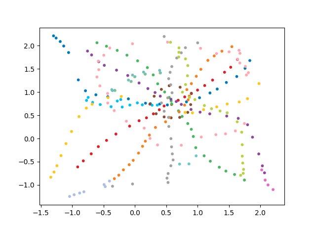
the version without text looks more beautiful and recognizable:
xn = fincoords[0][:,0] yn = fincoords[0][:,1] zn = fincoords[0][:,2] l=[labels[idi] for idi in myIDs] colors=[ccode[lines[idi]] for idi in myIDs] xyzn = zip(xn, yn, zn) fig = plt.figure() ax = fig.gca(projection='3d') ax.scatter(xn,yn,zn, c=colors, marker='o') plt.show()
UPD: Add metro lines of the desired color and create a gif. Black lines - transitions between stations:
myedges=[(myIDs.index(edge[0]),myIDs.index(edge[1]))for edge in G.edges] xn = fincoords[0][:,0] yn = fincoords[0][:,1] zn = fincoords[0][:,2] l=[labels[idi] for idi in myIDs] c=[ccode[lines[idi]] for idi in myIDs] fig = plt.figure() ax = fig.gca(projection='3d') ax.scatter(x,y,z, c=c, marker='o',s=25) for edge in myedges: col='black' if c[edge[0]]==c[edge[1]]: col=c[edge[0]] ax.plot3D([x[edge[0]], x[edge[1]]], [y[edge[0]], y[edge[1]]], [z[edge[0]], z[edge[1]]], col) ims = [] def rotate(angle): ax.view_init(azim=angle) rot_animation = animation.FuncAnimation(fig, rotate, frames=np.arange(0, 362, 3), interval=70) rot_animation.save('rotation2.gif', dpi=80, writer=matplotlib.animation.PillowWriter(80))
From this scheme, some interesting conclusions can be drawn that are not so obvious from other schemes. For some branches, for example, green, blue or violet, the MCC (pink ring) is practically useless due to uncomfortable transplants, which can be seen in the distance of the ring from these branches. The longest routes are from a communal apartment to a snapping or Pyatnitsky highway (red and pink / blue horses); long routes are also Alma-Ata storytelling and Bunin Alley-Nekrasovka. Judging by the plan, in the north of Moscow there is a partial duplication of gray and light green branches - they are nearby in the diagram. It would be interesting to see how the new lines (WDC, BKL) and who will use them more often. In any case, I hope such schemes can be interesting tools for analysis, inspiration and travel planning.
PS 3D is not necessary, for the 2D version it is enough to slightly correct the code. But in the case of the 2d scheme, it is impossible to achieve such accuracy of distances.
All Articles