This article is about a model based on the Bayesian network, which describes quotes of world currencies. Based on a simple metric, I will show that the pattern of behavior of world currency quotes over the past two years (from the beginning of 2018 to the end of 2019) coincides with that observed during the two years before the beginning of the acute phase of the global economic crisis of 2008. The results of my mini-study are in agreement with the opinion of many experts that today the world economy is on the verge of a large-scale economic crisis that could surpass the 2008 crisis. I will also describe how I built the model, where I took the data and give my analysis of the results of the model on the example of ruble quotes. I'll start with a small amount of technical details.
n-dimensional space of quotes
Quotes of world currencies for a certain period can be represented as a set of points in n-dimensional space, where n is the number of currencies in question. Each point in such a space is described by a vector of n elements. Elements of this vector are quotes values of n world currencies for one day. In other words, we have n axes on each of which we postpone the quote value of the corresponding currency.
Points in this multidimensional space are distributed in a certain way. Knowing this distribution, we can measure the probability of observation for each point. Thus, you can find points that have an abnormally low probability. That is, knowing the area of space where the point cloud for historical quotes is located, we can find the points that lie outside or on the border of this cloud.
Currency (or currencies) because of whose quotation our point (in n-dimensional space) is unlikely to be called overvalued or underestimated, depending on which direction along the axis of the corresponding currency this point has moved. If the currency has an abnormally large quotation, then we will call it overvalued, if it is anomalously small, then underestimated. Knowing that the currency is underestimated, we can assume that the likelihood of strengthening it in the near future is high and, conversely, if the currency is overvalued, then a scenario is likely to decrease in its value.
Reasons for abnormal quotes
The low probability of observing a point in our n-dimensional space indicates that at least one currency has an abnormally high or abnormally low quote value at a given time. In the general case, some or all currencies have such quotes, a combination of which in the n-dimensional vector was rarely observed or never was observed in the studied historical period. There are many reasons for this, but they are all characterized by the onset of the influence of certain factors that affect one or many currencies.
One of the reasons is a simple hypothetical example for the ruble. Suppose, as a result of the policy of the Central Bank of Russia (CB), there was an economically unjustified devaluation of the ruble. In this case, quotes that correspond to the devalued ruble will be located in n-dimensional space away from the cloud of points that were observed in the previous historical interval. That is, the points will lie in the region of space where the probability of observing them is small. We can only find a way how to measure this probability.
It should be noted that the economically unreasonable weakening or strengthening of the ruble can be caused both by the influence of strong players (the Central Bank, the Ministry of Finance, etc.) and the inertia of the currency when the trend still exists, but the economic factors that initiated it have little influence.
Bayesian network
To measure the probabilities for each point, a model is required that describes their distribution. As such a model, I chose the Bayesian network as it is easy to understand, use and can well describe the mutual dependencies between currencies. After training, such a model knows the fluctuation of which currency is the cause and which effect.
In fig. Figure 1 shows an example of a graph for five currencies. Ovals are currencies, and arrows show dependencies. Here, currency 1 depends on currency 2 and currency 3, currency 5 on currency 1 and currency 4, etc. If we describe this graph in terms of regression, then the dependence means that currency 1 is on the left side of the regression model, and currency 2 and currency 3 are on the right side. The same logic for currency 5 and for the rest.
Such a graph can be built by hand if you know the dependencies or (as I did) determine from the data using special algorithms. After training the Bayesian network on currency quotes, we get a graph similar to that in Fig. 1 and also the degree of influence of one currency on another.
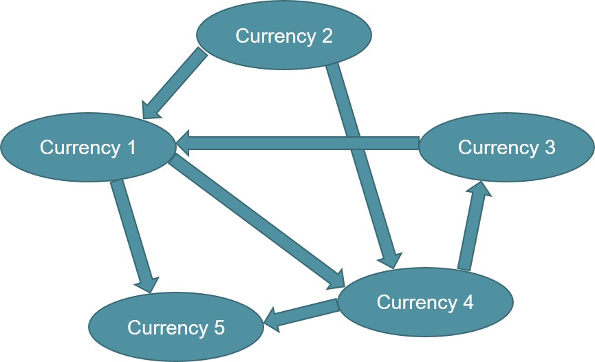
Figure 1. An example of a Bayesian network.
The Bayesian network gives us the opportunity to evaluate the likelihood for each currency quote. Credibility is a certain number that indicates how likely the existence of a given quote is for a given model. Credibility gives us information on how far (or how close) this quote is from the area where it is most likely to be expected in the quotes space. In other words, the likelihood of a quote on a particular day indicates how far the currency quote is from its expected value. That is, how much it is underestimated or overestimated.
Also, in addition to plausibility, the Bayesian network gives the value of the expected value of the quote. Thus, combining information about the likelihood of a quote, its expected and real values, we can tell on any day in the past (for example, yesterday) how much one currency or another is underestimated or overestimated.
If the real value of the currency is less than expected and the likelihood of a point is small, then the currency is underestimated. Conversely, if the real value of the currency is higher than expected and the likelihood is also small, then the currency is overvalued. For example, if the dollar price on the exchange is 65 rubles and the Bayesian network says that the likelihood of such a quote is small, and the expected value is 70 rubles per dollar, this means that the ruble is overvalued.
Bayes training
To train the model, I took quotes of currencies at the end of each trading day. The data on world currencies was taken for free from finance.yahoo.com. After a long purge (many missing values and emissions), I chose about 100 currencies that have a more or less informative distribution. That is, he rejected those currencies in which the exchange rate is regulated by direct administrative mechanisms. Such currencies have had the same exchange rate for years and only occasionally devalue in leaps and bounds. I must say that all currencies are somehow regulated by the Central Bank or the government, but there are some whose information content is obviously small for the model. Thus, in our n-dimensional space, n is 100.
After cleaning and other data processing, I trained the Bayesian network in R using the bnlearn package. The package is very convenient with a good description and works quickly. Quotes, although they are a time sequence, but entered the model without reference to time. Data has been used since 2003. For each next year, the model was overtrained using data for the entire previous period. That is, on January 1 of each year, the model trains again with the inclusion of new data accumulated for the previous year.
results
We are on the verge of a global crisis
In fig. Figure 2 shows the log-likelihood logarithm for each point in our 100-dimensional space of world currency quotes. The vertical axis represents the log-likelihood value, and the horizontal axis represents the date. The log-likelihood metric should be interpreted as follows: the lower its value, the less likely it is to observe world currency quotes on a given day. Extremely low values of this metric may indicate some large-scale changes in the global economy.
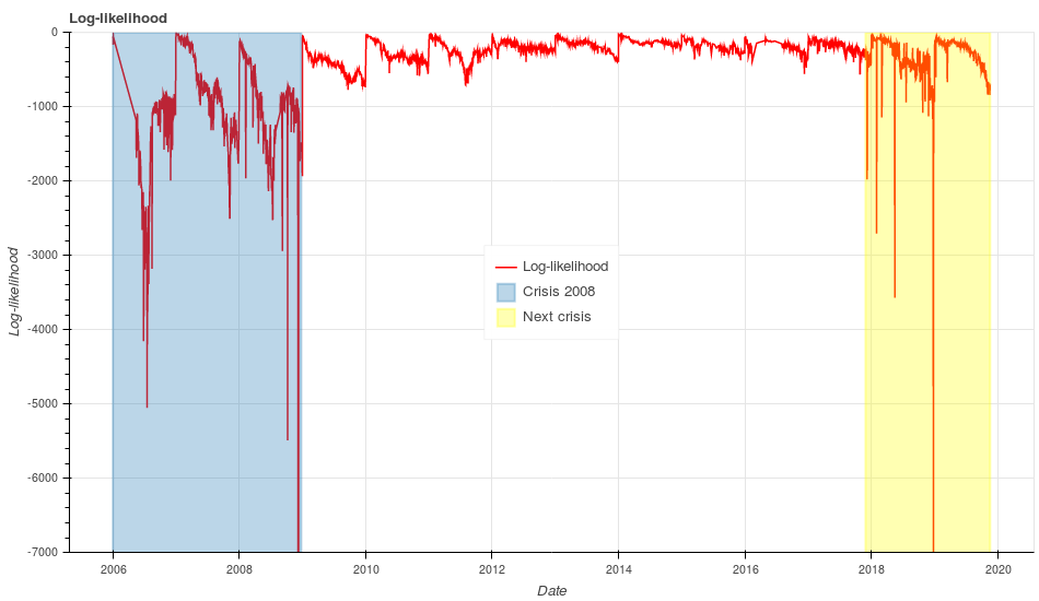
Figure 2: Probabilities (log-likelihood) to observe quotes of world currencies for each day (red lines). The area of crisis 2008 is highlighted in blue, the area of the beginning of a likely next crisis is highlighted in orange.
Let's pay attention to the region from 2006 to the end of 2008 (the region is highlighted in blue in Fig. 2). We see that the minimum log-likelihood values in this area are observed at the end of 2008. As we know, at this time there was an acute phase of the global economic crisis, accompanied by the collapse of a number of financial organizations, such as the investment bank Lehman Brothers.
In the previous two years from 2006 to 2007, we have seen significant fluctuations in log-likelihood. If we could return to the past in those years and look at this schedule, then we would definitely conclude that something extraordinary is happening in the global economy. Today we know that these spikes on the chart in 2006-2007 were the harbingers of the global economic crisis.
Now let's look at the current period from 2018 to the end of 2019 (the area is highlighted in orange in Fig. 2). After almost 8 years of relative calm, our log-likelihood metric again, as in 2006-2007, shows significant surges. Moreover, at the end of 2018, log-likelihood fell significantly lower than what was observed two years before the 2008 crisis. If in mid-2006 we observe a surge to -5000, then at the end of 2018 we observe a surge of -12000 (extremely low negative values are not shown in the graph )
This can most likely indicate the presence of large-scale changes in the global economy, similar to or even more significant than those two years before the 2008 crisis. Thus, if we compare the behavior of the metric today with its behavior in the 2008 crisis, we can assume that in the next For a year or two, the world economy will face big shocks that may surpass those of 2008.
Add a little clarity to the graph in Fig. 2. We see that for each year there is a steady downtrend from the beginning to the end of the year. The metric values are near zero at the beginning of the year due to the fact that the model is training anew at the beginning of each year and thus includes information on recent quotes. By the end of the year, the shape of the distribution of quotes in our n-dimensional space is changing. Due to the fact that the model does not know anything about the new distribution, it is expected to show low log-likelihood values for them.
This is underlined by the fact that the world economy is in continuous motion: new economic ties between countries appear and old ones disappear. That is, a uniform decrease in the metric from the beginning to the end of the year is the expected picture, and strong surges and a sharp decline indicate strong changes in the global economy.
Due to the log-likelihood’s downtrend, it’s difficult to apply it directly to assess how currencies are undervalued or overvalued. To do this, I introduced a new metric called z-value. The z-value metric depends on three values: the transformed log-likelihood (here log-likelihood for a particular currency, and not the one in Fig. 2), the expected value and the real value of currency quotes. Thus, z-value is a certain indicator of how undervalued or overvalued a currency is.
Let's look at the Russian ruble
Further, I will show that z-value relatively well indicates an increased probability of a trend change. Let's look at fig. 3 where quotes of the Russian ruble are depicted by green lines. The z-value metric is shown in the graph with red and blue dots. Red dots indicate that the ruble is overvalued, and blue dots indicate that the ruble is underestimated. The size of the points depends on the absolute value of z-value (the larger the value, the larger the point).
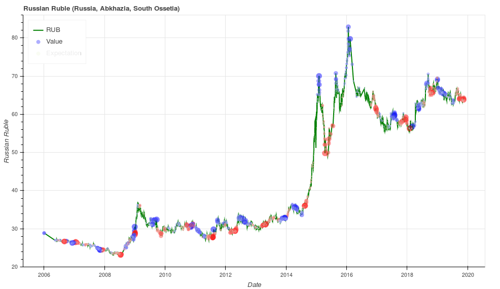
Figure 3: Overvaluation (red dots) and nonvaluation (blue dots) for ruble quotes (green lines)
Hereinafter, for ease of perception, I use the quotation value inverse to that adopted in the world of finance. This is due to the fact that for most people it is easier to remember how much a dollar in rubles costs than the inverse of it.
On the graph, we see that local minima are usually highlighted in red, and local maxima are usually highlighted in blue. Highs and lows are, obviously, points of trend change. There are areas (for example, the end of 2018) where the metric indicates a trend change, but the actual trend remains the same. Thus, the z-value metric indicates an increased likelihood of a trend change in the coming days or weeks.
Next, I will try to analyze the behavior of the expected values for the ruble quotes (expected ruble value). The expected value of the quote is the one that the Bayesian network expects on a specific day for a particular currency based on the quotes of the remaining 99 currencies. The Bayesian network knows everything about the distribution of quotes and, therefore, knows about their expected values.
Let's look at fig. 4, where ruble quotes are shown with green lines (as in the previous chart), and light green dots indicate the expected quotes that the Bayesian network gave us. I will try to give my interpretation of how the expected values of ruble quotes behave using two periods as an example.
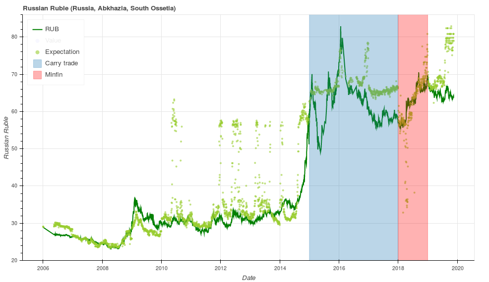
Figure 4: Ruble quotes (green lines) and its expected value (light green dots). The period where the carry trade strategy was popular was highlighted in blue. Pink color shows the area with remarkable activity of the Ministry of Finance of Russia.
Let's look at the period from the beginning of 2015 to the end of 2017, which is highlighted in blue in Fig. 4. We see that the expected value of the ruble is systematically much lower than the real value (light green dots are higher than dark green). During this period, the Central Bank will cancel the currency corridor, terminate interventions and sharply increase the key rate from 10% to 17% with a smooth subsequent decrease back to 10% (the key rate on the Central Bank website ). This situation gave a powerful impetus to carry trade operations, which attracted speculative capital and strengthened the ruble above a fundamentally sound level.
Carry trade is a trading strategy when, for example, you take a loan in Japan at 0.1% and put that money on a bank deposit in a Russian bank at 7%. After a year, you close the deposit, give the money to the Japanese bank along with interest, take the profit for yourself, which consists of the difference in interest rates between the Central banks of Japan and Russia.
Now let's look at 2018 (the area in Fig. 4 is highlighted in pink). Here I just want to share one of my observations. Since the beginning of the year, the Ministry of Finance of Russia (the Ministry of Finance) has been buying up foreign currency in the domestic foreign exchange market for an average of 15-20 billion rubles a day. At the end of August 2018, the Ministry of Finance completed these operations. If we look at fig. 4, we will see that throughout this period (from the beginning of 2018 to August 2018) the expected value of the ruble was higher than the real one and only in August (exactly when the Ministry of Finance stopped buying the currency) the points of the expected value on the charts became higher than the real (expected value , respectively, below).
It can be assumed that during this period some factors influenced the influx of currency into the country's economy, and the graph shows this high expected value of the ruble. Accordingly, the Ministry of Finance was able to withdraw this currency from circulation without much damage to the economy. The figures for the purchase of foreign currency by the ministry can be seen in the table on the Central Bank’s website , the fifth column (the column is called “the operations of the Ministry of Finance of Russia to purchase (sell) foreign currency in the domestic foreign exchange market *”)
Charts for other currencies
For those who want to analyze the behavior of other currencies, I made a website www.valuenetto.com , where you can look at the z-value metric and the expected values of all 100 currencies. The site is not intended for a large number of users, so it can sometimes slow down.
After going to the site, click the blue button in the upper right corner (where the “choose currency” prompt flashes) and select the currency that interests you (you can type the name of the country in the field that appears). Then a graph will appear similar to that in the previous two figures. The dial in the upper left shows the current z-value. If you click on the line below the dial, a detailed description for z-value will appear.
The site works automatically. At the end of each trading day, quotation data is uploaded. The model is asked likelihood for the currencies from which the z-value metric is calculated (shown as red and blue dots on the graphs). At the end of each year, the automatic model is trained anew taking into account new data for the previous year.
Once again about the global economic crisis
Many experts regularly warn of the imminent start of a new global economic crisis, which is expected to be much larger than what we saw before. The reason they see in the fundamental shortcomings of the modern capitalist model of the economy.
One of these experts, Martin Wolfe, argues that today's capitalism is “rentier capitalism” and rent is the main root of the ills of the global economy. The rent is understood as the excess income from the rental of a resource. Such a resource can be real estate or the professional qualities of a highly qualified specialist who works for hire for an unreasonably high salary.
Another expert, Mikhail Khazin, expresses the view that the existence of capitalism is possible only with constantly expanding markets and with ever-increasing consumption. Further expansion of the markets is impossible today due to the fact that as a result of globalization, global markets are more or less developed. An increase in consumption is also impossible due to the large debt burden of consumers in developed countries. This means that the time of capitalism is over and in the near future the world will begin the transition to a new economic model based on other principles. The transition will be accompanied by a significant decline in world consumption.
Thus, we all will probably witness big changes in the near future.
Disclaimer
The model described here is not a complete trading algorithm. The author does not guarantee that its use in automated trading systems will increase, reduce or not change the performance of such systems.
update:
1) Corrected grammatical errors. Thanks AndyPike , polearnik and sheru
2) Added a chapter to Disclaimer on the recommendation of bellerofonte