All the methods for solving the equation discussed here are based on the least squares method. We denote the methods as follows:
- Analytical solution
- Gradient descent
- Stochastic gradient descent
For each of the methods for solving the equation of the straight line, the article presents various functions that are mainly divided into those that are written without using the NumPy library and those that use NumPy for calculations. The skillful use of NumPy is believed to reduce computing costs.
All the code in this article is written in python 2.7 using the Jupyter Notebook . Source code and sample data file posted on Github
The article is more focused on both beginners and those who have already begun to master the study of a very extensive section in artificial intelligence - machine learning.
To illustrate the material, we use a very simple example.
Example conditions
We have five values that characterize the dependence of Y on X (Table No. 1):
Table No. 1 "Conditions of the example"
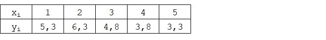
We assume that the values Is the month of the year, and - revenue this month. In other words, revenue depends on the month of the year, and - the only sign on which revenue depends.
An example is so-so, both in terms of the conditional dependence of revenue on the month of the year, and in terms of the number of values - there are very few of them. However, this simplification will allow what is called on the fingers to explain, not always with ease, the material absorbed by beginners. And also the simplicity of the numbers will allow, without significant labor costs, those who wish to solve the example on paper.
Suppose that the dependence shown in the example can be quite well approximated by the mathematical equation of a simple (pairwise) regression line of the form:
Where - this is the month in which the revenue was received, - revenue corresponding to the month, and - regression coefficients of the estimated line.
Note that the coefficient often called the slope or gradient of the estimated line; represents the amount by which to change when it changes .
Obviously, our task in the example is to select such coefficients in the equation and for which the deviations of our estimated monthly revenue from the true answers, i.e. values presented in the sample will be minimal.
Least square method
In accordance with the least squares method, the deviation should be calculated by squaring it. Such a technique avoids the mutual repayment of deviations, if they have opposite signs. For example, if in one case, the deviation is +5 (plus five), and in the other -5 (minus five), then the sum of the deviations will be mutually repaid and will be 0 (zero). You can not squander the deviation, but use the property of the module and then all deviations will be positive and will accumulate in us. We will not dwell on this point in detail, but simply indicate that for the convenience of calculations, it is customary to square the deviation.
This is how the formula looks with the help of which we determine the smallest sum of squared deviations (errors):
Where Is a function of approximating true answers (i.e., revenue calculated by us),
- these are true answers (revenue provided in the sample),
Is the sample index (the number of the month in which the deviation is determined)
We differentiate the function, define the partial differential equations, and are ready to proceed to the analytical solution. But first, let's take a short digression on what differentiation is and recall the geometric meaning of the derivative.
Differentiation
Differentiation is the operation of finding the derivative of a function.
What is a derivative for? The derivative of a function characterizes the rate of change of a function and indicates its direction. If the derivative at a given point is positive, then the function increases, otherwise, the function decreases. And the larger the value of the derivative modulo, the higher the rate of change of the values of the function, as well as the steeper the angle of the graph of the function.
For example, under the conditions of the Cartesian coordinate system, the value of the derivative at the point M (0,0) equal to +25 means that at a given point, when the value is shifted right per unit, value increases by 25 conventional units. On the graph, it looks like a fairly steep angle of rise of values from a given point.
Another example. A derivative value of -0.1 means that when offset per conventional unit, value decreases by only 0.1 conventional unit. At the same time, on the function graph, we can observe a barely noticeable tilt down. Drawing an analogy with the mountain, we seem to be very slowly descending the gentle slope from the mountain, unlike the previous example, where we had to take very steep peaks :)
Thus, after differentiating the function by coefficients and , we define the equations of partial derivatives of the first order. After determining the equations, we get a system of two equations, having solved which we can choose such values of the coefficients and at which the values of the corresponding derivatives at given points change by a very, very small value, and in the case of the analytical solution they do not change at all. In other words, the error function for the found coefficients reaches a minimum, since the values of the partial derivatives at these points will be zero.
So, according to the rules of differentiation, the equation of the partial derivative of the 1st order with respect to the coefficient will take the form:
1st order partial derivative equation with respect to will take the form:
As a result, we got a system of equations that has a fairly simple analytical solution:
\ begin {equation *}
\ begin {cases}
na + b \ sum \ limits_ {i = 1} ^ nx_i - \ sum \ limits_ {i = 1} ^ ny_i = 0
\\
\ sum \ limits_ {i = 1} ^ nx_i (a + b \ sum \ limits_ {i = 1} ^ nx_i - \ sum \ limits_ {i = 1} ^ ny_i) = 0
\ end {cases}
\ end {equation *}
Before solving the equation, pre-load, check the correct loading and format the data.
Download and format data
It should be noted that due to the fact that for the analytical solution, and later on for gradient and stochastic gradient descent, we will use the code in two variations: using the NumPy library and without using it, we will need to format the data accordingly (see the code).
Download and data processing code
# import pandas as pd import numpy as np import matplotlib.pyplot as plt import math import pylab as pl import random # Jupyter %matplotlib inline # from pylab import rcParams rcParams['figure.figsize'] = 12, 6 # Anaconda import warnings warnings.simplefilter('ignore') # table_zero = pd.read_csv('data_example.txt', header=0, sep='\t') # print table_zero.info() print '********************************************' print table_zero print '********************************************' # NumPy x_us = [] [x_us.append(float(i)) for i in table_zero['x']] print x_us print type(x_us) print '********************************************' y_us = [] [y_us.append(float(i)) for i in table_zero['y']] print y_us print type(y_us) print '********************************************' # NumPy x_np = table_zero[['x']].values print x_np print type(x_np) print x_np.shape print '********************************************' y_np = table_zero[['y']].values print y_np print type(y_np) print y_np.shape print '********************************************'
Visualization
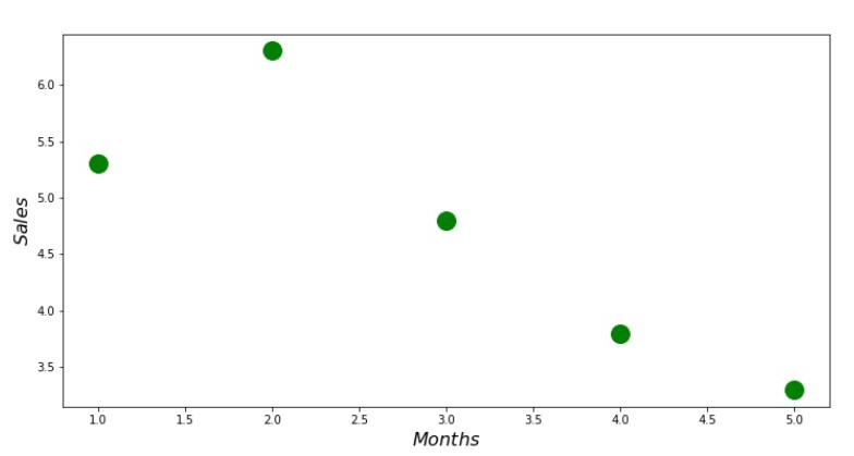
Now, after we, firstly, downloaded the data, secondly, we checked the correct loading and finally formatted the data, we will conduct the first visualization. Often, the pairplot method of the Seaborn library is used for this. In our example, due to the limited numbers, it makes no sense to use the Seaborn library. We will use the regular Matplotlib library and look only at the scatterplot.
Scatterplot Code
print ' №1 " "' plt.plot(x_us,y_us,'o',color='green',markersize=16) plt.xlabel('$Months$', size=16) plt.ylabel('$Sales$', size=16) plt.show()
Chart No. 1 “Dependence of revenue on the month of the year”
Analytical solution
We will use the most common tools in python and solve the system of equations:
\ begin {equation *}
\ begin {cases}
na + b \ sum \ limits_ {i = 1} ^ nx_i - \ sum \ limits_ {i = 1} ^ ny_i = 0
\\
\ sum \ limits_ {i = 1} ^ nx_i (a + b \ sum \ limits_ {i = 1} ^ nx_i - \ sum \ limits_ {i = 1} ^ ny_i) = 0
\ end {cases}
\ end {equation *}
By Cramer’s rule, we find a common determinant, as well as determinants by and by , after which, dividing the determinant by on the common determinant - we find the coefficient , similarly find the coefficient .
Analytical Solution Code
# a b def Kramer_method (x,y): # ( ) sx = sum(x) # ( ) sy = sum(y) # list_xy = [] [list_xy.append(x[i]*y[i]) for i in range(len(x))] sxy = sum(list_xy) # list_x_sq = [] [list_x_sq.append(x[i]**2) for i in range(len(x))] sx_sq = sum(list_x_sq) # n = len(x) # det = sx_sq*n - sx*sx # a det_a = sx_sq*sy - sx*sxy # a a = (det_a / det) # b det_b = sxy*n - sy*sx # b b = (det_b / det) # () check1 = (n*b + a*sx - sy) check2 = (b*sx + a*sx_sq - sxy) return [round(a,4), round(b,4)] # ab_us = Kramer_method(x_us,y_us) a_us = ab_us[0] b_us = ab_us[1] print '\033[1m' + '\033[4m' + " a b:" + '\033[0m' print 'a =', a_us print 'b =', b_us print # def errors_sq_Kramer_method(answers,x,y): list_errors_sq = [] for i in range(len(x)): err = (answers[0] + answers[1]*x[i] - y[i])**2 list_errors_sq.append(err) return sum(list_errors_sq) # error_sq = errors_sq_Kramer_method(ab_us,x_us,y_us) print '\033[1m' + '\033[4m' + " " + '\033[0m' print error_sq print # # print '\033[1m' + '\033[4m' + " :" + '\033[0m' # % timeit error_sq = errors_sq_Kramer_method(ab,x_us,y_us)
Here's what we got:
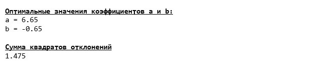
So, the coefficient values are found, the sum of the squared deviations is set. We draw a straight line on the scattering histogram in accordance with the coefficients found.
Regression line code
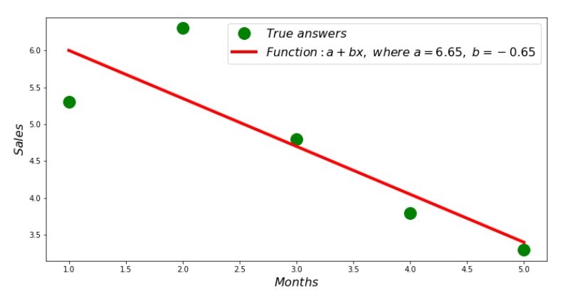
# def sales_count(ab,x,y): line_answers = [] [line_answers.append(ab[0]+ab[1]*x[i]) for i in range(len(x))] return line_answers # print '№2 " "' plt.plot(x_us,y_us,'o',color='green',markersize=16, label = '$True$ $answers$') plt.plot(x_us, sales_count(ab_us,x_us,y_us), color='red',lw=4, label='$Function: a + bx,$ $where$ $a='+str(round(ab_us[0],2))+',$ $b='+str(round(ab_us[1],2))+'$') plt.xlabel('$Months$', size=16) plt.ylabel('$Sales$', size=16) plt.legend(loc=1, prop={'size': 16}) plt.show()
Schedule No. 2 “Correct and Estimated Answers”
You can look at the deviation schedule for each month. In our case, we cannot take any significant practical value out of it, but we will satisfy the curiosity of how well the simple linear regression equation characterizes the dependence of revenue on the month of the year.
Deviation Schedule Code
# def error_per_month(ab,x,y): sales_c = sales_count(ab,x,y) errors_percent = [] for i in range(len(x)): errors_percent.append(100*(sales_c[i]-y[i])/y[i]) return errors_percent # print '№3 " -, %"' plt.gca().bar(x_us, error_per_month(ab_us,x_us,y_us), color='brown') plt.xlabel('Months', size=16) plt.ylabel('Calculation error, %', size=16) plt.show()
Schedule No. 3 “Deviations,%”
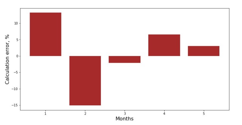
Not perfect, but we completed our task.
We write a function that, for determining the coefficients and uses the NumPy library, more precisely - we will write two functions: one using a pseudo-inverse matrix (not recommended in practice, since the process is computationally complex and unstable), the other using a matrix equation.
Analytical Solution Code (NumPy)
# 1. # , a vector_1 = np.ones((x_np.shape[0],1)) x_np = table_zero[['x']].values # x_np x_np = np.hstack((vector_1,x_np)) # , print vector_1[0:3] print x_np[0:3] print '***************************************' print # , a b def pseudoinverse_matrix(X, y): # X = np.matrix(X) # XT = XT # XTX = XT*X # inv = np.linalg.pinv(XTX) # y = np.matrix(y) # return (inv*XT)*y # ab_np = pseudoinverse_matrix(x_np, y_np) print ab_np print '***************************************' print # , def matrix_equation(X,y): a = np.dot(XT, X) b = np.dot(XT, y) return np.linalg.solve(a, b) # ab_np = matrix_equation(x_np,y_np) print ab_np
Compare the time taken to determine the coefficients and , in accordance with the 3 methods presented.
Code for calculating calculation time
print '\033[1m' + '\033[4m' + " NumPy:" + '\033[0m' % timeit ab_us = Kramer_method(x_us,y_us) print '***************************************' print print '\033[1m' + '\033[4m' + " :" + '\033[0m' %timeit ab_np = pseudoinverse_matrix(x_np, y_np) print '***************************************' print print '\033[1m' + '\033[4m' + " :" + '\033[0m' %timeit ab_np = matrix_equation(x_np, y_np)
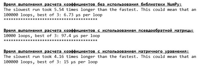
On a small amount of data, the “self-written” function comes forward, which finds the coefficients using the Cramer method.
Now you can move on to other ways of finding the coefficients and .
Gradient descent
First, let's define what a gradient is. In a simple way, a gradient is a segment that indicates the direction of the maximum growth of a function. By analogy with climbing uphill, where the gradient looks, there is the steepest climb to the top of the mountain. Developing the mountain example, we recall that in fact we need the steepest descent in order to reach the lowland as soon as possible, that is, the minimum - the place where the function does not increase or decrease. At this point, the derivative will be zero. Therefore, we need not a gradient, but an anti-gradient. To find the anti-gradient, you just need to multiply the gradient by -1 (minus one).
We draw attention to the fact that a function can have several minima, and going down to one of them according to the algorithm proposed below, we will not be able to find another minimum, which is possibly lower than the one found. Relax, we are not in danger! In our case, we are dealing with a single minimum, since our function on the graph is an ordinary parabola. And as we all should know very well from the school course of mathematics, the parabola has only one minimum.
After we found out why we needed the gradient, and also that the gradient is a segment, that is, a vector with given coordinates, which are exactly the same coefficients and we can implement gradient descent.
Before starting, I suggest reading just a few sentences about the descent algorithm:
- We determine the coordinates of the coefficients in a pseudo-random way and . In our example, we will determine the coefficients near zero. This is a common practice, but each practice may have its own practice.
- From coordinate subtract the value of the partial derivative of the 1st order at the point . So, if the derivative is positive, then the function increases. Therefore, taking away the value of the derivative, we will move in the opposite direction of growth, that is, in the direction of descent. If the derivative is negative, then the function at this point decreases and taking away the value of the derivative we move towards the descent.
- We carry out a similar operation with the coordinate : subtract the value of the partial derivative at the point .
- In order not to jump the minimum and not fly into far space, it is necessary to set the step size towards the descent. In general, you can write an entire article on how to correctly set the step and how to change it during the descent to reduce the cost of calculations. But now we have a slightly different task, and we will establish the step size by the scientific method of “poking” or, as they say in common people, empirically.
- After we are from the given coordinates and subtracted the values of the derivatives, we obtain new coordinates and . We take the next step (subtraction), already from the calculated coordinates. And so the cycle starts again and again, until the required convergence is achieved.
Everything! Now we are ready to go in search of the deepest gorge of the Mariana Trench. Getting down.
Gradient Descent Code
# NumPy. # x,y, ( =0,1), (tolerance) def gradient_descent_usual(x_us,y_us,l=0.1,tolerance=0.000000000001): # ( ) sx = sum(x_us) # ( ) sy = sum(y_us) # list_xy = [] [list_xy.append(x_us[i]*y_us[i]) for i in range(len(x_us))] sxy = sum(list_xy) # list_x_sq = [] [list_x_sq.append(x_us[i]**2) for i in range(len(x_us))] sx_sq = sum(list_x_sq) # num = len(x_us) # , a = float(random.uniform(-0.5, 0.5)) b = float(random.uniform(-0.5, 0.5)) # , 1 0 # errors = [1,0] # # , , tolerance while abs(errors[-1]-errors[-2]) > tolerance: a_step = a - l*(num*a + b*sx - sy)/num b_step = b - l*(a*sx + b*sx_sq - sxy)/num a = a_step b = b_step ab = [a,b] errors.append(errors_sq_Kramer_method(ab,x_us,y_us)) return (ab),(errors[2:]) # list_parametres_gradient_descence = gradient_descent_usual(x_us,y_us,l=0.1,tolerance=0.000000000001) print '\033[1m' + '\033[4m' + " a b:" + '\033[0m' print 'a =', round(list_parametres_gradient_descence[0][0],3) print 'b =', round(list_parametres_gradient_descence[0][1],3) print print '\033[1m' + '\033[4m' + " :" + '\033[0m' print round(list_parametres_gradient_descence[1][-1],3) print print '\033[1m' + '\033[4m' + " :" + '\033[0m' print len(list_parametres_gradient_descence[1]) print
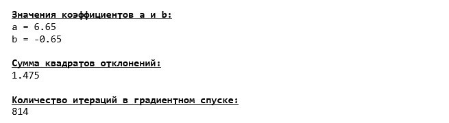
We plunged to the very bottom of the Mariana Trench and there we found all the same values of the coefficients and , which in fact was to be expected.
Let's make another dive, only this time, the filling of our deep-sea vehicle will be other technologies, namely the NumPy library.
Gradient Descent Code (NumPy)
# NumPy, # NumPy def error_square_numpy(ab,x_np,y_np): y_pred = np.dot(x_np,ab) error = y_pred - y_np return sum((error)**2) # NumPy. # x,y, ( =0,1), (tolerance) def gradient_descent_numpy(x_np,y_np,l=0.1,tolerance=0.000000000001): # ( ) sx = float(sum(x_np[:,1])) # ( ) sy = float(sum(y_np)) # sxy = x_np*y_np sxy = float(sum(sxy[:,1])) # sx_sq = float(sum(x_np[:,1]**2)) # num = float(x_np.shape[0]) # , a = float(random.uniform(-0.5, 0.5)) b = float(random.uniform(-0.5, 0.5)) # , 1 0 # errors = [1,0] # # , , tolerance while abs(errors[-1]-errors[-2]) > tolerance: a_step = a - l*(num*a + b*sx - sy)/num b_step = b - l*(a*sx + b*sx_sq - sxy)/num a = a_step b = b_step ab = np.array([[a],[b]]) errors.append(error_square_numpy(ab,x_np,y_np)) return (ab),(errors[2:]) # list_parametres_gradient_descence = gradient_descent_numpy(x_np,y_np,l=0.1,tolerance=0.000000000001) print '\033[1m' + '\033[4m' + " a b:" + '\033[0m' print 'a =', round(list_parametres_gradient_descence[0][0],3) print 'b =', round(list_parametres_gradient_descence[0][1],3) print print '\033[1m' + '\033[4m' + " :" + '\033[0m' print round(list_parametres_gradient_descence[1][-1],3) print print '\033[1m' + '\033[4m' + " :" + '\033[0m' print len(list_parametres_gradient_descence[1]) print
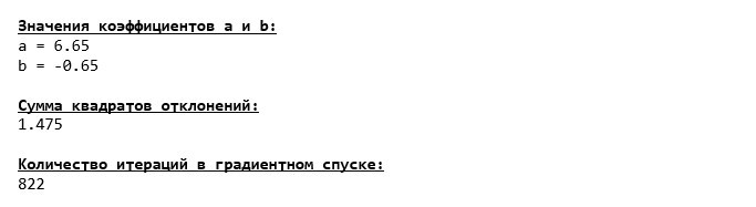
Coefficient Values and unchanging.
Let's look at how the error changed during gradient descent, that is, how the sum of the squared deviations changed with each step.
Code for the graph of the sums of the squared deviations
print '№4 " -"' plt.plot(range(len(list_parametres_gradient_descence[1])), list_parametres_gradient_descence[1], color='red', lw=3) plt.xlabel('Steps (Iteration)', size=16) plt.ylabel('Sum of squared deviations', size=16) plt.show()
Chart №4 “The sum of the squares of deviations in the gradient descent”
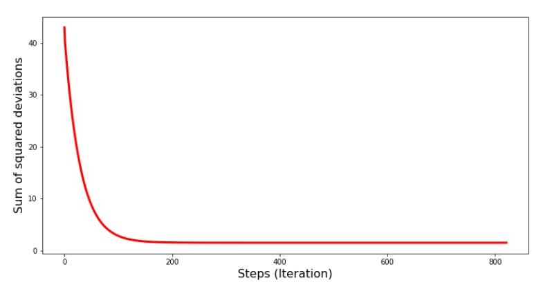
On the graph we see that with each step the error decreases, and after a certain number of iterations we observe an almost horizontal line.
Finally, we estimate the difference in the execution time of the code:
Code for determining the gradient descent calculation time
print '\033[1m' + '\033[4m' + " NumPy:" + '\033[0m' %timeit list_parametres_gradient_descence = gradient_descent_usual(x_us,y_us,l=0.1,tolerance=0.000000000001) print '***************************************' print print '\033[1m' + '\033[4m' + " NumPy:" + '\033[0m' %timeit list_parametres_gradient_descence = gradient_descent_numpy(x_np,y_np,l=0.1,tolerance=0.000000000001)
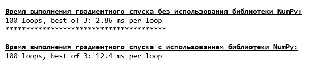
Perhaps we are doing something wrong, but again, a simple "self-written" function that does not use the NumPy library is ahead of the time using the function using the NumPy library.
But we do not stand still, but move towards the study of another exciting way to solve the equation of simple linear regression. Meet me!
Stochastic gradient descent
In order to quickly understand the principle of operation of stochastic gradient descent, it is better to determine its differences from ordinary gradient descent. We, in the case of gradient descent, in the equations of derivatives of and used the sum of the values of all attributes and the true answers available in the sample (i.e., the sum of all and ) In stochastic gradient descent, we will not use all the values available in the sample, but instead, in a pseudo-random way, we will choose the so-called sample index and use its values.
For example, if the index is determined by the number 3 (three), then we take the values and , then we substitute the values in the equations of derivatives and determine the new coordinates. Then, having determined the coordinates, we again pseudo-randomly determine the index of the sample, substitute the values corresponding to the index in the partial differential equations, and determine the coordinates in a new way and etc. before
What are the advantages of stochastic gradient descent over the usual? If our sample size is very large and measured in tens of thousands of values, then it is much easier to process, say a random thousand of them than the entire sample. In this case, the stochastic gradient descent is launched. In our case, of course, we will not notice a big difference.
We look at the code.
Code for stochastic gradient descent
# .. def stoch_grad_step_usual(vector_init, x_us, ind, y_us, l): # , ind # (.- stoch_grad_descent_usual) x = x_us[ind] # y (), x y_pred = vector_init[0] + vector_init[1]*x_us[ind] # error = y_pred - y_us[ind] # ab grad_a = error # ab grad_b = x_us[ind]*error # vector_new = [vector_init[0]-l*grad_a, vector_init[1]-l*grad_b] return vector_new # .. def stoch_grad_descent_usual(x_us, y_us, l=0.1, steps = 800): # vector_init = [float(random.uniform(-0.5, 0.5)), float(random.uniform(-0.5, 0.5))] errors = [] # # (steps) for i in range(steps): ind = random.choice(range(len(x_us))) new_vector = stoch_grad_step_usual(vector_init, x_us, ind, y_us, l) vector_init = new_vector errors.append(errors_sq_Kramer_method(vector_init,x_us,y_us)) return (vector_init),(errors) # list_parametres_stoch_gradient_descence = stoch_grad_descent_usual(x_us, y_us, l=0.1, steps = 800) print '\033[1m' + '\033[4m' + " a b:" + '\033[0m' print 'a =', round(list_parametres_stoch_gradient_descence[0][0],3) print 'b =', round(list_parametres_stoch_gradient_descence[0][1],3) print print '\033[1m' + '\033[4m' + " :" + '\033[0m' print round(list_parametres_stoch_gradient_descence[1][-1],3) print print '\033[1m' + '\033[4m' + " :" + '\033[0m' print len(list_parametres_stoch_gradient_descence[1])
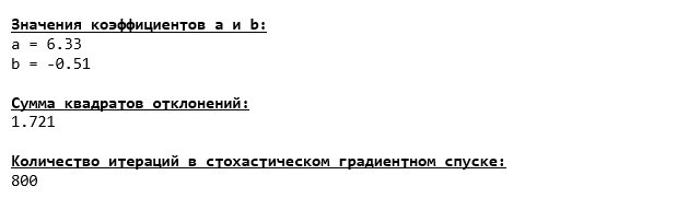
We look carefully at the coefficients and catch ourselves on the question “How so?”. We got other values of the coefficients and . Maybe stochastic gradient descent found more optimal parameters of the equation? Unfortunately no. It is enough to look at the sum of the squared deviations and see that with the new values of the coefficients, the error is greater. Do not rush to despair. We plot the error change.
Code for the graph of the sum of the squared deviations in stochastic gradient descent
print ' №5 " -"' plt.plot(range(len(list_parametres_stoch_gradient_descence[1])), list_parametres_stoch_gradient_descence[1], color='red', lw=2) plt.xlabel('Steps (Iteration)', size=16) plt.ylabel('Sum of squared deviations', size=16) plt.show()
Chart №5 “The sum of the squared deviations in the stochastic gradient descent”
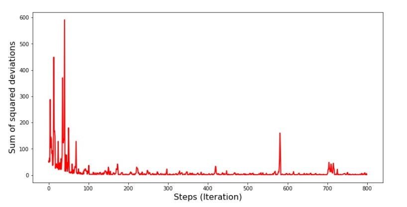
Having looked at the schedule, everything falls into place and now we will fix everything.
So what happened? The following happened.When we randomly select a month, it is for the selected month that our algorithm seeks to reduce the error in calculating revenue. Then we select another month and repeat the calculation, but we reduce the error already for the second month selected. And now recall that in our first two months we deviate significantly from the line of the equation of simple linear regression. This means that when any of these two months is selected, then reducing the error of each of them, our algorithm seriously increases the error throughout the sample. So what to do?The answer is simple: you need to reduce the descent step. After all, having reduced the step of descent, the error will also cease to “jump” now up and down. Rather, the error “skip” will not stop, but it will not do so quickly :) We’ll check.
Code to run SGD in less steps
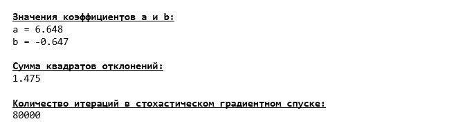
# , 100 list_parametres_stoch_gradient_descence = stoch_grad_descent_usual(x_us, y_us, l=0.001, steps = 80000) print '\033[1m' + '\033[4m' + " a b:" + '\033[0m' print 'a =', round(list_parametres_stoch_gradient_descence[0][0],3) print 'b =', round(list_parametres_stoch_gradient_descence[0][1],3) print print '\033[1m' + '\033[4m' + " :" + '\033[0m' print round(list_parametres_stoch_gradient_descence[1][-1],3) print print '\033[1m' + '\033[4m' + " :" + '\033[0m' print len(list_parametres_stoch_gradient_descence[1]) print ' №6 " -"' plt.plot(range(len(list_parametres_stoch_gradient_descence[1])), list_parametres_stoch_gradient_descence[1], color='red', lw=2) plt.xlabel('Steps (Iteration)', size=16) plt.ylabel('Sum of squared deviations', size=16) plt.show()
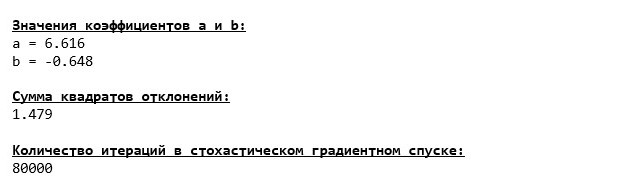
Chart №6 “The sum of the squared deviations in the stochastic gradient descent (80 thousand steps)”
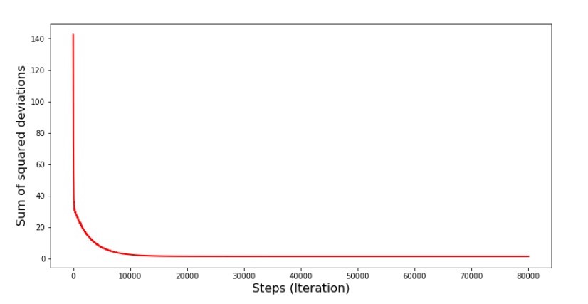
The values of the coefficients improved, but still not ideal. Hypothetically, this can be corrected in this way. For example, at the last 1000 iterations, we choose the values of the coefficients with which the minimal error was made. True, for this we will have to write down the coefficient values themselves. We will not do this, but rather pay attention to the schedule. It looks smooth, and the error seems to decrease evenly. This is actually not the case. Let's look at the first 1000 iterations and compare them with the last.
Code for SGD chart (first 1000 steps)
print ' №7 " -. 1000 "' plt.plot(range(len(list_parametres_stoch_gradient_descence[1][:1000])), list_parametres_stoch_gradient_descence[1][:1000], color='red', lw=2) plt.xlabel('Steps (Iteration)', size=16) plt.ylabel('Sum of squared deviations', size=16) plt.show() print ' №7 " -. 1000 "' plt.plot(range(len(list_parametres_stoch_gradient_descence[1][-1000:])), list_parametres_stoch_gradient_descence[1][-1000:], color='red', lw=2) plt.xlabel('Steps (Iteration)', size=16) plt.ylabel('Sum of squared deviations', size=16) plt.show()
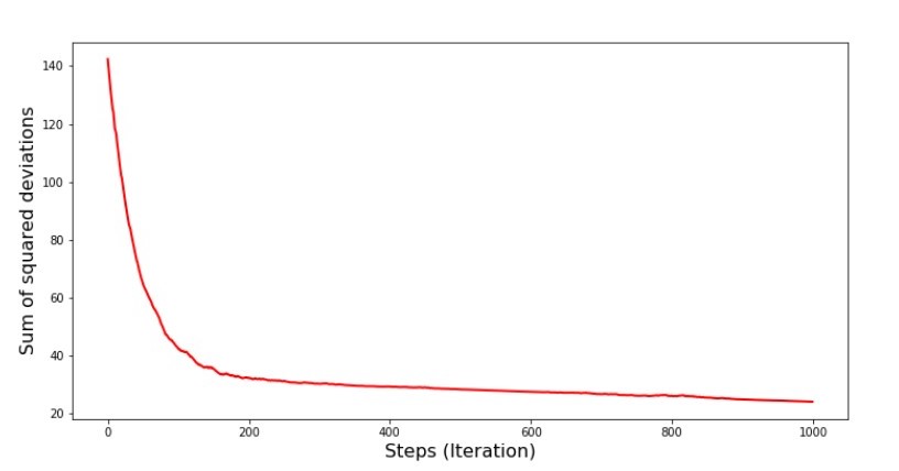
Schedule No. 7 “The sum of the squares of the deviations of the SGD (first 1000 steps)”
Graph No. 8 “The sum of the squares of the deviations of the SGD (last 1000 steps)”
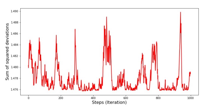
At the very beginning of the descent we observe a fairly uniform and sharp decrease in the error. At the last iterations, we see that the error goes around and around a value of 1.475 and at some points even equals this optimal value, but then it goes up anyway ... I repeat, we can write down the values of and , and then select those for which the error is minimal. However, we had a more serious problem: we had to take 80 thousand steps (see code) to get values close to optimal. And this already contradicts the idea of saving computational time with stochastic gradient descent relative to gradient. What can be corrected and improved? It is not difficult to notice that at the first iterations we confidently go down and, therefore, we should leave a big step in the first iterations and reduce the step as we move forward. We will not do this in this article - it has already dragged on. Those who wish can themselves think how to do it, it’s not difficult :)
Now we will perform a stochastic gradient descent using the NumPy library (and we won’t stumble over the stones that we identified earlier)
Code for stochastic gradient descent (NumPy)
# def stoch_grad_step_numpy(vector_init, X, ind, y, l): x = X[ind] y_pred = np.dot(x,vector_init) err = y_pred - y[ind] grad_a = err grad_b = x[1]*err return vector_init - l*np.array([grad_a, grad_b]) # def stoch_grad_descent_numpy(X, y, l=0.1, steps = 800): vector_init = np.array([[np.random.randint(X.shape[0])], [np.random.randint(X.shape[0])]]) errors = [] for i in range(steps): ind = np.random.randint(X.shape[0]) new_vector = stoch_grad_step_numpy(vector_init, X, ind, y, l) vector_init = new_vector errors.append(error_square_numpy(vector_init,X,y)) return (vector_init), (errors) # list_parametres_stoch_gradient_descence = stoch_grad_descent_numpy(x_np, y_np, l=0.001, steps = 80000) print '\033[1m' + '\033[4m' + " a b:" + '\033[0m' print 'a =', round(list_parametres_stoch_gradient_descence[0][0],3) print 'b =', round(list_parametres_stoch_gradient_descence[0][1],3) print print '\033[1m' + '\033[4m' + " :" + '\033[0m' print round(list_parametres_stoch_gradient_descence[1][-1],3) print print '\033[1m' + '\033[4m' + " :" + '\033[0m' print len(list_parametres_stoch_gradient_descence[1]) print
The values turned out to be almost the same as during the descent without using NumPy . However, this is logical.
We will find out how much time stochastic gradient descents took us.
Code for determining SGD calculation time (80 thousand steps)
print '\033[1m' + '\033[4m' +\ " NumPy:"\ + '\033[0m' %timeit list_parametres_stoch_gradient_descence = stoch_grad_descent_usual(x_us, y_us, l=0.001, steps = 80000) print '***************************************' print print '\033[1m' + '\033[4m' +\ " NumPy:"\ + '\033[0m' %timeit list_parametres_stoch_gradient_descence = stoch_grad_descent_numpy(x_np, y_np, l=0.001, steps = 80000)
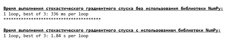
The farther into the forest, the darker the clouds: again the “self-written" formula shows the best result. All this suggests that there should be even more subtle ways to use the NumPy library , which really accelerate the operations of calculations. In this article we will not find out about them. There will be something to think about at your leisure :)
Summarize
Before summarizing, I would like to answer the question that most likely arose from our dear reader. Why, in fact, such “torment” with descents, why do we have to go up and down the mountain (mainly down) to find the treasured lowland, if we have such a powerful and simple device in our hands, in the form of an analytical solution that instantly teleports us to Right place?
The answer to this question lies on the surface. We have now examined a very simple example in which the true answer depends on one sign .In life, this is not often seen, so imagine that we have signs of 2, 30, 50 or more. Add to this thousands, or even tens of thousands of values for each attribute. In this case, the analytical solution may not pass the test and fail. In turn, gradient descent and its variations will slowly but surely bring us closer to the goal - the minimum of the function. And do not worry about speed - we’ll probably also analyze ways that will allow us to set and adjust the step length (i.e. speed).
And now actually a brief summary.
Firstly, I hope that the material presented in the article will help beginners "date Scientists" in understanding how to solve the equations of simple (and not only) linear regression.
Secondly, we examined several ways to solve the equation. Now, depending on the situation, we can choose the one that is best suited to solve the problem.
Thirdly, we saw the power of additional settings, namely the step length of the gradient descent. This parameter cannot be neglected. As noted above, in order to reduce the cost of calculations, the step length should be changed along the descent.
Fourth, in our case, “self-written” functions showed the best temporal result of calculations. This is probably due to not the most professional use of the capabilities of the NumPy library. But be that as it may, the conclusion is as follows. On the one hand, sometimes it is worth questioning established opinions, and on the other hand, it is not always worth complicating things — on the contrary, sometimes a simpler way to solve a problem is more effective. And since our goal was to analyze three approaches in solving the equation of simple linear regression, the use of “self-written” functions was quite enough for us.
Literature (or something like that)
1. Linear regression
http://statistica.ru/theory/osnovy-lineynoy-regressii/
2. Least square method
mathprofi.ru/metod_naimenshih_kvadratov.html
3. Derivative
www.mathprofi.ru/chastnye_proizvodnye_primery.html
4. Gradient
math /proizvodnaja_po_napravleniju_i_gradient.html
5. Gradient descent
habr.com/en/post/471458
habr.com/en/post/307312
artemarakcheev.com//2017-12-31/linear_regression
6. NumPy library
docs.scipy.org/doc/ numpy-1.10.1 / reference / generated / numpy.linalg.solve.html
docs.scipy.org/doc/numpy-1.10.0/reference/generated/numpy.linalg.pinv.html
pythonworld.ru/numpy/2. html