Splines in 3d graphics, the most automated option

About a month ago, I began to learn Python from the book of Dawson and woke up deeply in the process of writing his game under pygame. TK was such that it seemed most promising to make a game with pseudo-three-dimensional graphics by stuffing the saved surfaces of 3d splines into sprites. I’ll write about the latter.



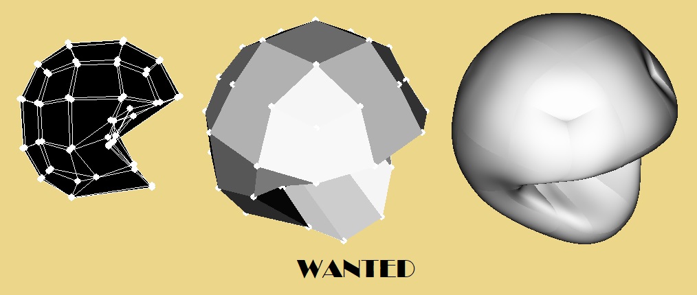
So, there are polygons (it is easiest to work with quadrangles) on which we want to stretch cubic surfaces so that they fit together quite smoothly - these surfaces are splines.







It is most convenient to present a spline for one polygon as a function

$$

$$g (u, v) = v \ cdot g_1 (u) + (1 - v) \ cdot g_2 (u) + u \ cdot g_3 (v) + (1-u) \ cdot g_4 (v) (1)$$

Here

$$

$$g_1, g_2, g_3, g_4$$

- cubic polynomials satisfying some boundary conditions (in the figure below - light green and red curves, and derivative-initial conditions - lilac and blue vectors); u and v vary from 0 to 1.







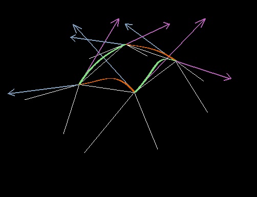
In this interpretation, some degrees are lost (products of 2 and 3 degrees of parameters), but the polynomial coefficients can be found by specifying only 12 vectors of initial conditions (4 polygon points and derivative vectors with respect to u and v for each point). At the junctions, splines coincide if similar initial conditions are set for neighboring polygons (the derivative vectors must be collinear, the surface passes through the same points of the polygon).



One misfortune - the derivative with such a statement of the problem on the entire border may not coincide - there will be small artifacts at the junctions. You can think up 4 more conditions for correcting this and carefully add another term to the formula

$$

$$u \ cdot v \ cdot (u-1) \ cdot (v-1) \ cdot g_5 (u, v)$$

which does not spoil the borders, but this is a topic for a separate article.



An alternative is the Bezier surface , but it proposes to set 16 parameters of incomprehensible (to me) mathematical meaning, i.e. it is assumed that the artist will work with his own hands. This is not very suitable for me, so a bicycle with crutches follows.



Coefficients (1) are most easily calculated by finding the inverse matrix to the matrix of values ​​and derivatives in the corners and multiplying by the input conditions (three times, for each coordinate). The matrix can be like this:





NumPy does an excellent job of this.



One question remains - where to get the vectors of derivatives. It is assumed that we must somehow choose them based on the position of neighboring (for the polygon) points and for reasons of smoothness.

For me personally, it was still completely counterintuitive how to deal with the length of the derivative vector. The direction is understandable, but the length?



As a result, the following algorithm was born:



1. At the first stage, some classification of points occurs. In the graph (which the polygon points and their connections specify), cycles of length 4 are searched and stored, and in addition, neighbors that are most suitable for the continuation of the edges of the polygon are recorded (it is determined in advance which edges correspond to a change in the parameter u and which correspond to v). Here is a piece of code that searches, sorts, and remembers neighbors for the 0th point of a cycle:





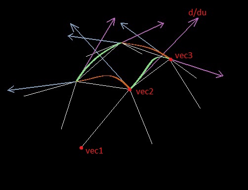
Further, when constructing the spline, the derivative along the edge (for example, with respect to the parameter u) at the point of the polygon is selected based on the location of two points of the edge and one neighboring point (let it be the points vec1, vec2 and vec3; the point at which the derivative is sought is the second).







At first I tried to use the normalized vector vec3 - vec1 (like I applied the Lagrange theorem) for this role, but problems arose with the length of the vector of derivatives - making it a constant was a bad idea.



Lyrical digression:



For a small illustration of what the derivative vector is in the parametric version, we turn to a simple two-dimensional analogy - here is a piece of a circular arc:

$$

$$g (u) = (Rsin (u \ pi / 2), Rcos (u \ pi / 2))$$

$$

$$g '(u) = (R \ pi / 2 \ cdot cos (u \ pi / 2), -R \ pi / 2 \ cdot sin (u \ pi / 2))$$

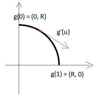
Those. derivative modulus = R * pi / 2 and, generally speaking, depends on the size of the piece of the arc, which we set through the parameter.



What to do now with this? Leo Nikolaevich Tolstoy bequeathed to us that everything is round = good, therefore, if we set the derivative at a point as if we would like to build an arc there, we will get a smooth beautiful curve.



The end of the digression.



The second stage of the derivative search:



2. Through our three points vec1, vec2, vec3 we build a plane, in this plane we look for a circle that passes through all three points. The desired derivative will be directed along the tangent to the circle at vec2, and the modulus of the vector of the derivative should be equal to the product of the radius of the circle and the angle of the sector, which form two points of the polygon face (similar to our simple flat analogy from the lyrical digression).

$$

$$g '= R \ cdot \ phi$$

Everything seems to be simple, here is the function code, for example (NumPy is used again):





Well, in general, it all somehow works. For demonstration, I took a 5x5x5 cube and changed the position of the points with a randomizer: