
Bayes theorem is one of the most famous theorems in statistics and probability theory. Even if you are not working with calculating quantitative indicators, you probably had to get acquainted with this theorem at some point in preparation for the exam.
P (A | B) = P (B | A) * P (A) / P (B)
That's how it looks, but what does it mean and how does it work? Today we will find out and delve into Bayes's theorem.
Reasons to confirm our judgment
What is the whole point of probability theory and statistics? One of the most important uses relates to decision making under uncertainty. When you decide to perform an action (unless, of course, you are a reasonable person), you bet that after the completion of this action it will entail a better result than if this action did not happen ... But betting is a thing unreliable, how do you ultimately decide whether to take this or that step or not?
One way or another, you evaluate the probability of a successful outcome, and if this probability is above a certain threshold value, you take a step.
Thus, the ability to accurately assess the likelihood of success is critical to making the right decisions. Despite the fact that randomness will always play a role in the final outcome, you should learn to use these randomnesses correctly and turn them to your advantage over time.
It is here that Bayes' theorem comes into force - it gives us a quantitative basis for maintaining our faith in the outcome of the action as environmental factors change, which, in turn, allows us to improve the decision-making process over time.
We analyze the formula
Let's look at the formula again:
P (A | B) = P (B | A) * P (A) / P (B)
Here:
- P (A | B) - probability of occurrence of event A, provided that event B has already happened;
- P (B | A) - probability of occurrence of event B, provided that event A has already happened. Now it looks like some kind of vicious circle, but we will soon understand why the formula works;
- P (A) - a priori (unconditional) probability of occurrence of event A;
- P (B) - a priori (unconditional) probability of occurrence of event B.
P (A | B) is an example of a posteriori (conditional) probability, that is, one that measures the probability of a certain state of the surrounding world (namely, the state in which event B occurred). Whereas P (A) is an example of a priori probability, which can be measured in any state of the surrounding world.
Let's look at Bayes' theorem in action by way of example. Suppose you recently completed a data analysis course from bootcamp. You have not received a response from some of the companies in which you were interviewed, and begin to worry. So, you want to calculate the likelihood that a particular company will make you a job offer, provided that three days have passed and they have not called you back.
We rewrite the formula in terms of our example. In this case, outcome A ( Offer ) is the receipt of a job offer, and outcome B ( NoCall ) is “no phone call for three days.” Based on this, our formula can be rewritten as follows:
P ( Offer | NoCall ) = P ( NoCall | Offer ) * P ( Offer ) / P ( NoCall )
The value of P ( Offer | NoCall ) is the probability of receiving an offer, provided that there is no call within three days. This probability is extremely difficult to assess.
However, the inverse probability, P ( NoCall | Offer ) , that is, the absence of a phone call for three days, given that in the end you received a job offer from the company, it is quite possible to attach some value. From conversations with friends, recruiters and consultants, you will find out that this probability is small, but sometimes a company can still remain silent for three days if it is still planning to invite you to work. So you evaluate:
P ( NoCall | Offer ) = 40%
40% is not bad and it seems there is still hope! But we are not done yet. Now we need to evaluate P ( Offer ) , the probability of going to work. Everyone knows that finding a job is a long and difficult process, and you may have to go through an interview several times before you receive this offer, so you evaluate:
P ( Offer ) = 20%
Now we just have to evaluate P ( NoCall ) , the probability that you will not receive a call from the company within three days. There are many reasons why you may not be called back within three days - they may reject your candidacy or still conduct interviews with other candidates, or the recruiter is simply ill and therefore does not call. Well, there are many reasons why you might not have a call, so you assess this probability as:
P ( NoCall ) = 90%
And now, putting it all together, we can calculate P ( Offer | NoCall ) :
P ( Offer | NoCall ) = 40% * 20% / 90% = 8.9%
This is quite small, so, unfortunately, it is more rational to leave hope for this company (and continue to send resumes to others). If it still seems a bit abstract, don't worry. I felt the same way when I first learned about Bayes' theorem. Now let's see how we came to these 8.9% (keep in mind that your initial 20% score was already low).
The intuition behind the formula
Remember, we talked about the fact that Bayes's theorem gives reason to confirm our judgments? So where do they come from? They are taken from the a priori probability P (A) , which in our example is called P ( Offer ) , in fact, this is our initial judgment on how likely it is that a person will receive a job offer. In our example, you can assume that a priori probability is the probability that you will receive a job offer at the very moment you leave the interview.
New information appears - 3 days have passed, and the company did not call you back. Thus, we use other parts of the equation to adjust our a priori probability of a new event.
Let's look at the probability P (B | A) , which in our example is called P ( NoCall | Offer ) . When you first see the Bayesian theorem, you wonder: How to understand where to get the probability P (B | A) ? If I don’t know what the probability of P (A | B) is , then in what magical way should I find out what the probability of P (B | A) is ? I recall the phrase Charles Munger once said:
“Flip, always flip!”
- Charles Munger
He meant that when you are trying to solve a difficult problem, you need to turn it upside down and look at it from a different angle. This is exactly what Bayes's theorem does. Let's reformulate Bayes' theorem in terms of statistics in order to make it more understandable (I learned about this from here ):

For me, for example, such a record looks clearer. We have an a priori hypothesis (Hypothesis) - that we got a job, and observed facts - evidence (Evidence) - there is no phone call for three days. Now we want to know the likelihood that our hypothesis is correct, taking into account the facts presented. As decided above, we have a probability of P (A) = 20% .
Time to turn everything upside down! We use P ( Evidence | Hypothesis ) to look at the problem from the other side and ask: “What is the probability of these evidence events occurring in a world where our hypothesis is true?” So, if we return to our example, we want to know how likely it is that if they do not call us within three days, we will still be hired. In the image above, I marked P ( Evidence | Hypothesis ) as “scaler” (scaler), because this word reflects the essence of the meaning well. When we multiply it by an a priori value, it decreases or increases the probability of an event, depending on whether any event proving our hypothesis is “harmful”. In our case, the more days pass without a call, the less likely we will be called to work. 3 days of silence is already bad (they reduce our a priori probability by 60%), while 20 days without a call will completely destroy the hope of getting a job. Thus, the more evidence events accumulate (more days pass without a phone call), the faster the scaler reduces the likelihood. A scaler is a mechanism that Bayes' theorem uses to adjust our judgment.
There is one thing that I struggled with in the original version of this article. It was a statement of why P ( Evidence | Hypothesis ) is easier to evaluate than P (Hypothesis | Evidence). The reason for this is that P ( Evidence | Hypothesis ) is a much more limited area of judgment about the world. Narrowing the scope, we simplify the task. We can draw an analogy with fire and smoke, where fire is our hypothesis, and the observation of smoke is an event proving the presence of fire. P (fire | smoke) is more difficult to evaluate, because a lot of things can cause smoke - car exhaust, factories, the person who fries hamburgers on charcoal. At the same time, P (smoke | fire) is easier to evaluate, because in a world where there is fire, there will almost certainly be smoke.
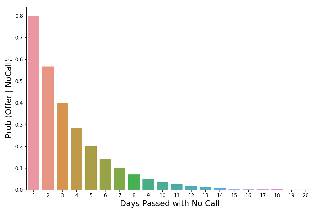
The probability value decreases as the number of days passes without a call.
The last part of the formula, P (B) or P ( Evidence ) , is the normalizer. As the name implies, its goal is to normalize the product of a priori probability and scaler. If there wasn’t a normalizer, we would have the following expression:

Note that the product of a priori probability and a scaler is equal to the joint probability. And since one of the components of P ( Evidence ) in it , then the joint probability would be affected by the small frequency of events.
This is a problem because shared probability is a value that includes all the states of the world. But we don’t need all the states, we need only those states that were confirmed by events-evidence. In other words, we live in a world where events - evidence has already taken place, and their number does not matter (therefore, we do not want them to affect our calculations in principle). Dividing the product of a priori probability and scaler by P ( Evidence ) changes it from joint probability to conditional (posterior). Conditional probability takes into account only those states of the world in which an event-proof occurred, which is exactly what we are achieving.
Another point of view from which we can look at why we divide the scaler into a normalizer is that they answer two important questions - and their relationship combines this information. Let's take an example from my recent Bayes article . Suppose we are trying to find out if the observed animal is a cat, based on a single sign - dexterity. All we know is that the animal we are talking about is agile.
- Scaler tells us what percentage of cats are good with dexterity. This value should be quite high, say 0.90.
- The normalizer tells us what percentage of animal traps in principle. This value should be average, say 0.50.
- The ratio 0.90 / 0.50 = 1.8 indicates that you need to change the a priori probability, because if you previously thought otherwise, it is time to change your mind, since you are most likely dealing with a cat. The reason why this can be thought of is that we observed some evidence that the animal is agile. Then we found that the proportion of dexterous cats is greater than the proportion of dexterous animals in general. Considering that at the moment we know only such evidence, and nothing more, it would be reasonable to reconsider our beliefs in the direction of thoughts that we are still watching a cat.
Summarize
Now that we know how to interpret each part of the formula, we can finally put everything together and look at what happened:
- Immediately after the interview, we establish an a priori probability - the chance that we will be hired is 20%.
- The more days that pass without a call, the less likely it is that we will be hired. For example, after three days without a call, we believe that in a world where we can get this job, there is only a 40% chance that the company will pull so long before it calls you. Multiply the scaler by an a priori probability and get 20% * 40% = 8%
- Finally, we understand that 8% was calculated for all conditions in which the world may be. But we are only concerned about conditions where we have not been called for three days. In order to work only with these conditions, we take for 90% the a priori probability that there will be no call within three days and we get a normalizer. We divide the previously received 8% into the normalizer 8% / 90% = 8.9% and get the final answer. Total, under all conditions of the world, if you have not received a call from the company within three days, the probability of getting a job is only 8.9%.
I hope this article has been helpful to you!