Variational Inference - what is it and what does it eat?

Hello, Habr!



Recently I talked with colleagues about a variational auto-encoder and it turned out that many even those working in Deep Learning know about the variational inference (Variational Inference) and, in particular, the Lower variational boundary only by hearsay and do not fully understand what it is.

In this article I want to analyze these issues in detail. Who cares, I ask for a cut - it will be very interesting.

What is variational inference?

The family of variational methods of machine learning got its name from the section of mathematical analysis “Variational calculus”. In this section, we study the problems of searching for extrema of functionals (a functional is a function of functions - that is, we are not looking for the values ​​of variables in which the function reaches its maximum (minimum), but such a function in which the functional reaches a maximum (minimum).



But the question arises - in machine learning, we always look for a point in the space of parameters (variables) in which the loss function has a minimum value. That is, it is the task of classical mathematical analysis, and here is the calculus of variations? The calculus of variations appears at the moment when we transform the loss function into another loss function (often this is the lower variational boundary) using the methods of calculus of variations.



Why do we need this? Is it not possible to directly optimize the loss function? We need these methods when it is impossible to directly obtain an unbiased gradient estimate (or this estimate has a very high dispersion). For example, our model sets $$$p (z)$ and $$$p (x / z)$ , and we need to calculate $$$p (x) = \ int (p (z) p (x / z) dz)$ . This is exactly what the variational auto encoder was designed for.

What is the Variational Lower Bound?

Imagine we have a function $$$f (x)$ . The lower bound on this function will be any function $$$g (x)$ satisfying the equation:

$$

$$g (x) <= f (x)$$

That is, for any function there are innumerable lower bounds. Are all of these lower bounds the same? Of course not. We introduce another concept - discrepancy (I did not find an established term in Russian-language literature, this value is called tightness in English-language articles):

$$

$$\ delta = max {f (x)} - max {g (x)}$$

Obviously enough, the residual is always positive. The smaller the residual, the better.



Here is an example of a lower bound with zero residual:



And here is an example with a small but positive residual:



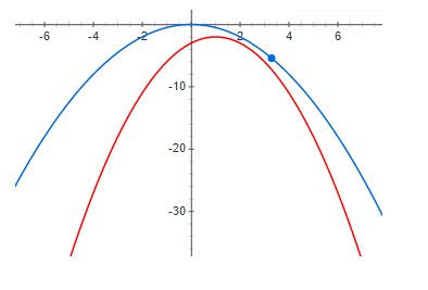
And finally, a big enough discrepancy:





From the above graphs, it is clearly seen that at zero residual, the maximum of the function and the maximum of the lower boundary are at the same point. That is, if we want to find the maximum of some function, we can search for the maximum of the lower boundary. If the discrepancy is not zero, then this is not so. And the maximum of the lower boundary can be very far (along the x axis) from the desired maximum. The graphs show that the larger the residual, the farther the highs can be from each other. This is generally not true, but in most practical cases this intuition works very well.

Variable Auto Encoder

Now we will analyze an example of a very good lower variational boundary with a potentially zero residual (below it will be clear why) - this is a Variational Autoencoder.



Our task is to build a generative model and train it using the maximum likelihood method. The model will look like this:

$$

$$q (x) = \ int {q (z) q_ \ theta (x | z) dz}$$

Where $$$q (x)$ Is the probability density of the generated samples, $$$z$ - latent variables, $$$q (z)$ - the probability density of a latent variable (often a simple one - for example, a multidimensional Gaussian distribution with zero expectation and unit dispersion - in general, something we can easily sample from), $$$q_ \ theta (x | z)$ - conditional sample density for a given value of latent variables, in the variational autoencoder, a Gaussian one with mat expectation and dispersion depending on z is selected.



Why might we need to represent data density in such a complex way? The answer is simple - the data has a very complex density function and we simply cannot technically construct a model of such a density directly. We hope that this complex density can be well approximated using two simpler densities. $$$q (z)$ and $$$q_ \ theta (x | z)$ .



We want to maximize the following function:

$$

$$I = \ int {p (x) log (q (x)) dx}$$

Where $$$p (x)$ - data probability density. The main problem is that the density $$$q (x)$ (with sufficiently flexible models) it is not possible to present analytically, and accordingly to train the model.



We use the Bayes formula and rewrite our function as follows:

$$

$$I = \ int {p (x) log (\ frac {q (z) q (x | z)} {q (z | x)}) dx}$$

Unfortunately, $$$q (z / x)$ everything is also difficult to calculate (it is impossible to take the integral analytically). But firstly, we note that the expression under the logarithm does not depend on z, so we can take the mathematical expectation from the logarithm in z of any distribution and this will not change the value of the function and multiply and divide by the logarithm by the same distribution (formally we have only one condition - this distribution should not vanish anywhere). As a result, we get:

$$

$$I = \ int {p (x) dx \ int {\ phi (z | x) log (\ frac {q (z) q (x | z)} {\ phi (z | x)})}} + \ int {p (x) dx \ int {\ phi (z | x) log (\ frac {\ phi (z | x)} {q (z | x)})}}$$

note that, firstly, the second term is KL divergence (which means it is always positive):

$$

$$I = \ int {p (x) dx \ int {\ phi (z | x) log (\ frac {q (z) q (x | z)} {\ phi (z | x)})}} + \ int {p (x) KL [\ phi (z | x) || q (z | x))] dx}$$

and secondly $$$I$ does not depend on $$$q (z | x)$ not from $$$\ phi (z | x)$ . It follows that,

$$

$$I> = \ int {p (x) dx \ int {\ phi (z | x) log (\ frac {q (z) q (x | z)} {\ phi (z | x)})}} = VLB$$

Where $$$Vlb$ - The lower variational boundary (Variational Lower Bound) and reaches its maximum when $$$KL [\ phi (z | x) || q (z | x))] = 0$ - i.e. the distributions are the same.



Positivity and equality to zero if and only if the distributions coincide KL-divergences are proved precisely by variational methods - hence the name of the variational boundary.



I want to note that the use of a variational lower bound gives several advantages. Firstly, it gives us the opportunity to optimize the loss function by gradient methods (try to do this when the integral is not analytically taken) and secondly, it approximates the inverse distribution $$$q (z | x)$ distribution $$$\ phi (z | x)$ - that is, we can not only sample data, but also sample latent variables. Unfortunately, the main drawback is when the inverse distribution model is not flexible, i.e., when the family $$$\ phi (z | x)$ does not contain $$$q (z | x)$ - the residual will be positive and equal:

$$

$$\ delta = \ int {p (x) \ underset {\ phi (z | x)} {min} (KL [\ phi (z | x) || q (z | x)]) dx}$$

and this means that the maximum of the lower boundary and the loss functions most likely do not coincide. By the way, the variational auto encoder used to generate pictures generates images that are too blurry, I think this is just because of choosing a too poor family $$$\ phi (z | x)$ .

An example of a not-so-good bottom line

Now we will consider an example where, on the one hand, the lower boundary has all the good properties (with a sufficiently flexible model, the residual will be zero), but in turn does not give any advantage over using the original loss function. I believe that this example is very revealing and if you do not do theoretical analysis, you can spend a lot of time trying to train models that make no sense. Rather, models make sense, but if we can train such a model, then it’s easier to choose $$$q (x)$ from the same family and use the maximum likelihood principle directly.



So, we will consider the exact same generative model as in the case of a variational auto encoder:

$$

$$q (x) = \ int {q (z) q_ \ theta (x | z) dz}$$

We will be training with the same method of maximum likelihood:

$$

$$I = \ int {p (x) log (q (x)) dx}$$

We still hope that $$$q (x | z)$ it will be much "easier" than $$$q (x)$ .

Only now we will write $$$I$ a little different:

$$

$$I = \ int {p (x) log (\ int {q (z) q_ \ theta (x | z) dz}) dx}$$

using the Jensen formula, we get:

$$

$$I> = \ int {p (x) q (z) log (q_ \ theta (x | z)) dxdz} = VLB$$

It is precisely at this moment that most people respond without thinking that this is really the lower limit and you can train the model. This is true, but let's look at the discrepancy:

$$

$$\ delta = \ int {p (x) log (q (x)) dx} - \ int {p (x) q (z) log (q_ \ theta (x | z)) dxdz}$$

where (by applying the Bayes formula twice):

$$

$$\ delta = \ int {p (x) q (z) log (\ frac {q (x)} {q (x | z)}) dxdz} = \ int {p (x) q (z) log ( \ frac {q (z)} {q (z | x)}) dxdz}$$

it is easy to see that:

$$

$$\ delta = \ int {p (x) KL [q (z) || q (z | x)] dx}$$

Let's see what happens if we increase the lower boundary - the residual will decrease. With a fairly flexible model:

$$

$$KL [q (z) || q (z | x)] \ rightarrow0$$

everything seems to be fine - the lower boundary has a potentially zero residual and with a fairly flexible model $$$q (x | z)$ everything should work. Yes, this is true, only attentive readers can notice that zero residual is achieved when $$$x$ and $$$z$ are independent random variables !!! and for a good result, the “complexity” of distribution $$$q (x | z)$ should be no less than $$$q (x)$ . That is, the lower border does not give us any advantages.

findings

The lower variational boundary is an excellent mathematical tool that allows you to approximately optimize "inconvenient" functions for learning. But like any other tool, you need to very well understand its advantages and disadvantages and also use it very carefully. We considered a very good example - a variational auto-encoder, as well as an example of a not very good lower boundary, while the problems of this lower boundary are difficult to see without a detailed mathematical analysis.



I hope it was at least a little useful and interesting.