Moreover, there is every reason to believe that the indicator Y depends on the indicator X. This position can be both a scientific hypothesis and be based on elementary common sense. For example, take grocery stores.
Denote by:
X - sales area (sq. M.)
Y - annual turnover (million p.)
Obviously, the higher the trading area, the higher the annual turnover (we assume a linear relationship).
Imagine that we have data on some n stores (retail space and annual turnover) - our dataset and k retail space (X), for which we want to predict annual turnover (Y) is our task.
We hypothesize that our value of Y depends on X in the form: Y = a + b * X
To solve our problem, we must choose the coefficients a and b.
First, let us set a and b random values. After that, we need to determine the loss function and the optimization algorithm.
To do this, we can use the root mean square loss function ( MSELoss ). It is calculated by the formula:
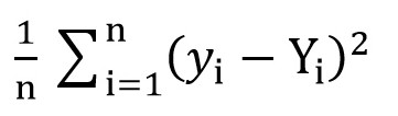
Where y [i] = a + b * x [i] after a = rand () and b = rand (), and Y [i] is the correct value for x [i].
At this stage, we have the standard deviation (a certain function of a and b). And it is obvious that the smaller the value of this function, the more precisely the parameters a and b are selected with respect to those parameters that describe the exact relationship between the area of the commercial premises and the turnover in this premises.
Now we can start using gradient descent (just to minimize the loss function).
Gradient descent
Its essence is very simple. For example, we have a function:
y = x*x + 4 * x + 3
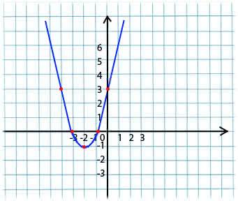
We take an arbitrary value of x from the domain of definition of the function. Imagine that this is the point x1 = -4.
Next, we take the derivative with respect to x of this function at the point x1 (if the function depends on several variables (for example, a and b), then we need to take partial derivatives with respect to each of the variables). y '(x1) = -4 <0
Now we get a new value for x: x2 = x1 - lr * y '(x1). The lr (learning rate) parameter allows you to set the step size. Thus we get:
If the partial derivative at a given point x1 <0 (the function decreases), then we move to the point of local minimum. (x2 will be larger than x1)
If the partial derivative at a given point x1> 0 (the function increases), then we are still moving to the point of local minimum. (x2 will be less than x1)
By performing this algorithm iteratively, we will approach the minimum (but will not reach it).
In practice, this all looks much simpler (however, I don’t presume to say which coefficients a and b fit the most accurately with the above case with shops, so we take a dependence of the form y = 1 + 2 * x to generate the dataset, and then train our model on this dataset):
(The code is written here )
import numpy as np # np.random.seed(42) # np- 1000 0..1 sz = 1000 x = np.random.rand(sz, 1) # y = f(x) y = 1 + 2 * x + 0.1 * np.random.randn(sz, 1) # 0 999 idx = np.arange(sz) # np.random.shuffle(idx) train_idx = idx # x_train, y_train = x[train_idx], y[train_idx] # a = np.random.randn(1) b = np.random.randn(1) print(a,b) # lr = 0.01 # n_epochs = 10000 # for epoch in range(n_epochs): # a b # yhat = a + b * x_train # 1. # : error = (y_train - yhat) # 2. ( ) # a a_grad = -2 * error.mean() # b b_grad = -2 * (x_train * error).mean() # 3. , a = a - lr * a_grad b = b - lr * b_grad print(a,b)
Having compiled the code, you can see that the initial values of a and b were far from the required values of 1 and 2, respectively, and the final values are very close.
I’ll clarify a little bit of why a_grad and b_grad are considered that way.
F(a, b) = (y_train - yhat) ^ 2 = (1 + 2 * x_train – a + b * x_train)
. The partial derivative of F with respect to a will be
-2 * (1 + 2 * x_train – a + b * x_train) = -2 * error
. The partial derivative of F with respect to b will be
-2 * x_train * (1 + 2 * x_train – a + b * x_train) = -2 * x_train * error
. We take the mean value
(mean())
since
error
and
x_train
and
y_train
are arrays of values, a and b are scalars.
Materials used in the article:
towardsdatascience.com/understanding-pytorch-with-an-example-a-step-by-step-tutorial-81fc5f8c4e8e
www.mathprofi.ru/metod_naimenshih_kvadratov.html