We are restoring a vintage (1969, judging by the chip marking) computer recently found by one of our employees. Analog computers were once popular for quick scientific calculations, but almost died out in the 1970s. They are interesting in a paradigm that is completely different from digital computers. In this post, I will focus on the operational amplifiers (op amps) used in this analog computer, Model 240 from Simulators Inc.

Model 240 Analog Computer by Simulators Inc. - “general-purpose high-precision analog desktop computer” containing up to 24 op-amps (there are 20 in this model).
What is an analog computer?
An analog computer performs calculations using physical, continuously variable values, such as voltage. In contrast to this, a digital computer uses discrete binary values. Analog computers have a long history - this includes gear mechanisms, logarithms , mechanical disk-ball integrators , tidal computers , and mechanical guidance systems. However, the “classic” analog computers of the 1950s and 1960s use op amps and integrators to solve differential equations. Usually they were programmed by connecting the wires to the patch panel, which led to the appearance of a mishmash of wires.

“Programming” analog computers by connecting wires to the patch panel. This panel is from an EAI analog computer
The great advantage of analog computers was their speed. They calculated results almost instantly, as their components worked in parallel. Digital computers sometimes needed to puff over computing for a long time. As a result, analog computers were most useful in real-time simulations. The disadvantage of analog computers was that their accuracy directly depended on the accuracy of their components; if you needed accuracy to 4 digits, you needed expensive resistors with an accuracy of 0.01%. At the same time, digital computers can be done with any accuracy, simply using more bits. Unfortunately for analog computers, the speed and power of digital computers grew exponentially, and by the 1970s there was practically no reason to use analog.
Inside an analog computer
The heart of an analog computer is its operational amplifiers (op amps). The opamps can summarize and scale the input signal, providing the simplest mathematical calculations. More importantly, by combining an op-amp with an accurate capacitor, integrators could be created. The integrator integrated the input over time, charging the capacitor. This allowed analog computers to solve differential equations. It may seem strange that integration, a complex mathematical operation, was the basic building block of analog computers, but that was how the hardware worked.

Analog computer integrators used large precision capacitors. At the top you can see a variable (customizable) capacitor at 10 nF, and a large metal box at the bottom is a variable capacitor at 10 uF. These capacitors were made so that the leakage was extremely small, and the integrable value did not leak out of them. In the foreground is a relay for selecting capacitors.
Analog computers used several potentiometers to set input values and scaling constants. To ensure high tuning accuracy, the potentiometers can be rotated up to 10 times. To check the potentiometers, a voltmeter was used. It could also be used to demonstrate output values, but more often they were displayed on an oscilloscope, chart tape, or plotter.
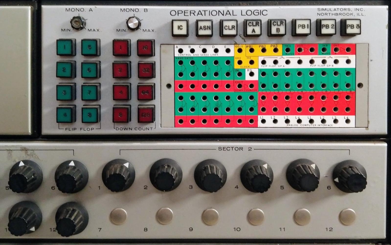
Above is the digital section of an analog computer. At the bottom are potentiometers; This computer model does not have some potentiometers. Instead of a blank panel, a digital voltmeter could be on the top left.
Some analog computers also had digital components — valves, triggers, monostable multivibrators, and counters. Such functionality made it possible to conduct more complex calculations - for example, iterate over solutions in the space of solutions. Our computer has a bit of digital logic that can be accessed through the color patch panel (pictured above).
In the photo below, the computer is partially disassembled. Inside, it turned out to be more complex than I expected, with many circuit boards. We removed the patch panel, which opened a grid of contacts to us. A cable connected to the patch panel closes the contacts and sets up the program. Five modules were found behind the panel on the computer: the leftmost one is removed and lies in front of the computer (in general, there is space for six modules inside, but one was not installed - apparently this is a cheaper model, and therefore it has not installed several potentiometers). The board, which is visible at the top, supports digital logic and two analog multipliers. Power and front panel circuits are located at the bottom.
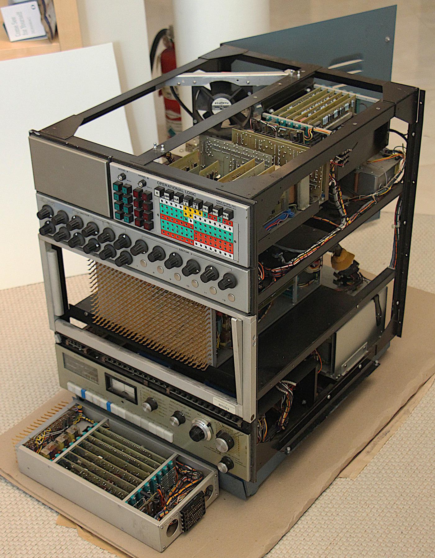
Analog computer with cover removed. One of the modules is removed and lies in front of it.
Below is a close-up photo of the module, as well as the contacts of the panel in front. Eight boards are visible behind. From left to right on the boards: four op amps (4 boards), various circuits (1 board) and a multiplier (3 boards). In an analog computer, multiplication was unexpectedly difficult to implement; Three boards are needed for a single circuit that multiplies two values.
Analog computers could calculate arbitrary functions using diode-resistor networks. For multiplication, the networks were tuned to calculate a parabolic function. Multiplication was considered through the identity X × Y = ((X + Y) 2 - (XY) 2 ) / 4. The sums and differences were calculated by means of the op-amp, and the square through the generator of the parabolic function.

One of the modules. “Fingers” on the front contacts are inserted into the patch panel. Behind them are visible square high-precision resistors (0.01%).
Operational amplifiers
In the photo above, each op-amp has its own separate board, filled with various components. Each board has an op-amp integrated circuit, which makes us wonder why so many other components are needed. The answer is simple - analog computers required very clear operation of the op-amp. In particular, the opamps had to work with signals at a constant current and low frequency, but, unfortunately, the opamps behave very poorly in this range, they like high frequencies more.
In 1949, a solution was developed for the operation of the op-amp at low frequencies: chopper amplifiers. The idea is this: the chopper modulates the input signal, say, at 400 Hz. The op-amp joyfully amplifies this alternating signal at 400 Hz. The second chopper demodulates the output variable signal back to constant, which gives much better results than direct amplification of a constant signal. The boards for the op-amp in an analog computer add a chopper circuit, complementing the integrated circuit of the op-amp and improving the quality of its operation.
The work of the chopper can be imagined as the work of an amplitude amplifier AM radio signal. True, unlike AM, demodulation must be “phase-sensitive” in order to distinguish between a positive and a negative signal.
The diagram (from this brochure ) shows the diagram of the op-amp board. The idea is that part of the input signal passes through a capacitor (high-pass filter) into an AC amplifier. Also, the input goes to the “stabilizing DC amplifier”, at the input of which there is a chopper. The output is demodulated and passes through a low-pass filter (resistor / capacitor). The two outputs of the amplifier are combined and are included in the "DC amplifier", the output amplifier.
Pay attention to the elements to recognize and prevent overload. In an analog computer, overload can happen quite easily when the calculated value is higher than expected and goes beyond the op-amp (± 10 V). As a result, the results will be incorrect. The op-amp catches overload and lights a light on the panel so that the user knows what the problem is. An important part of the work of an analog computer programmer is to understand how to scale the data so that the mathematical values fit into the physical limitations of the system.

The diagram below shows one of the op-amp boards. Today, an op-amp usually has a positive and negative input, but analog computers usually only had a negative input - so they summarized the data and inverted it. On the right you can see the entrance (separated from all other contacts on the left to avoid noise). The entrances are divided into three tracks. The first leads to a DC chopper amplifier. The signal passes through a low-pass filter to extract direct current and low-frequency signal. The chopper is simple: a field effect transistor with a JFET PN junction alternately ground the signal under the control of an external 400 Hz oscillator. Such a modulated signal is supplied to the Amelco 809 op amp IC, which appeared in 1967 (the Amelco company, now forgotten, once played an important role in the production of op amp; in particular, it made the first JFET op amp). IP is a round metal cylinder; then such cases were popular, and helped shield the op-amp from noise. Finally, the output of the IC passes through a second chopper and a filter for demodulation.
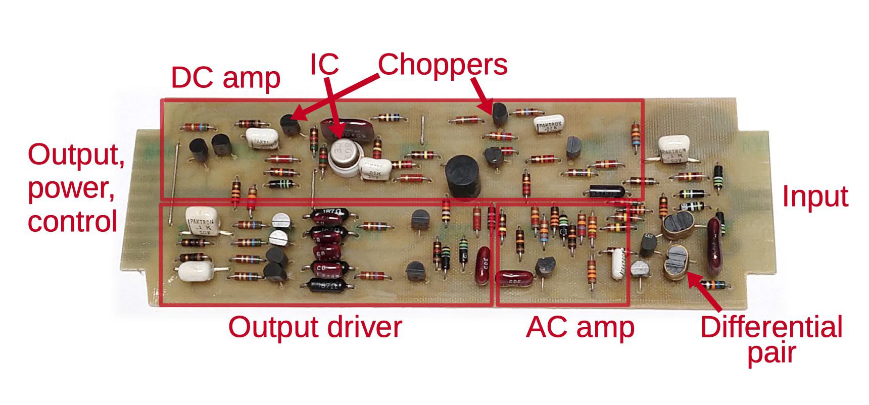
OA board from an analog computer, with marked up functional groups. Although the board uses an op-amp with ICs, an additional kit is required to achieve the required operational efficiency of the op-amp.
There are contacts on the left side, and here is the result of my reverse engineering of the board:
L: balance in
K: chopper ground
J: overload signal out
H: chopper drive in
F: ground
E: ground
D: -15V
C: + 15V
B: op amp output
A: unused
Then the second input track is combined with the output of the DC amplifier. Most op amps use a differential pair, and this board is no exception. In a differential pair, two transistors give a large gain to the difference between the two incoming signals. The input signals of the differential pair are the input signal of the board and the signal from the DC chopper amplifier, so it amplifies both the initial input and the constant signal. For the op-amp to work correctly, the two transistors in the differential pair must be perfectly balanced. In particular, transistors must operate at the same temperature, so they are connected by a metal clip.

Important transistors are connected with a metal clip so that they work at the same temperature. Differential pair on the right and on the left are the input transistor buffers.
The third input track goes to the AC amplifier. The incoming signal passes through a high-pass filter (resistor and capacitor), and then through a simple transistor buffer. The “forward propagation” signal is combined with the output of the differential pair to improve the frequency response of the amplifier. At this point, the input signal is amplified in three different ways, which gives good quality at both low and high frequencies.
The last stage of the op-amp board is an output amplifier that gives a strong current, which is used in the rest of the computer. It is an AB class amplifier. At that time, individual transistors lacked power, so it uses two NPN transistors and two PNP transistors.
Each board has an input and output connected to a patch panel. Below in the photo, the op-amp panels (from A1 to A4) are in the form of pieces of cake; their entrances are green and the exits are red. The op-amps used in integrators are also connected to integrating capacitors.

Close-up of a patch panel with connectors for A1, A3 and A4. The entrances are green, the exits are red. Initial conditions IC are white. Potentiometer connectors yellow.
On the patch panel, each op-amp has several input connectors with different resistor values for scaling; these are numbers 10 and 100 in the photo. The photo below shows these high-precision resistors (black cylinders) directly connected to the contacts of the patch panel. Integrator inputs are controlled by relays (below) and electronic switches so that the analog computer can initialize the integrating capacitors, start the calculation and save the result for analysis.

Resistors (black cylinders) are directly connected to the terminals of the patch panel. The relays in the middle control various states of the computer: initial conditions, operation, and retention. The boards connect to the green pins below.
Conclusion
Although integrated circuits with op-amps existed in the late 1960s, their quality was not enough for analog computers. Instead, for each op-amp, a whole board with components was used, combining the op-amp ICs with choppers and other elements, which made it possible to implement a high-precision op-amp. Although improvements in the quality of ICs have led to an exponential increase in the speed of computing digital computers, analogue computers have, in comparison with them, extremely small advantages from IPs. As a result, digital computers have won, and analog computers today are only historical artifacts.

Removable patch panel for an analog computer. It was programmed by connecting wires through the holes. The panel can be removed, so while one programmer used a computer, another could connect wires at that time.
I describe the circuit of an analog computer in such detail because we are trying to restore it, but we lack documentation. Therefore, I am engaged in reverse engineering, trying to understand how to restore it to working condition and how to program it. Although the circuit diagrams of the boards are quite simple, the computer has a lot of components that need to be analyzed. The hardest thing is to understand the connections in tight bundles of wires, and basically it is necessary to do this with a multimeter.