Euler-Poisson integral. Details on calculation methods

In the article, in detail, down to the smallest detail, three methods of taking the Euler-Poisson integral are considered. In one of the methods, an auxiliary reduction formula is derived. To find some complex integrals, one can use reduction formulas that reduce the degree of the integrand and calculate the corresponding integrals in a finite number of steps.



This integral is taken from the Gaussian function: $$$I = \ int \ limits_0 ^ \ infty {e ^ {- x ^ 2} dx}$

There is a very interesting mathematical way. To find the original integral, first look for the square of this integral, and then take the root from the result. Why? Yes, because it is much easier and painless to go to the polar coordinates. Therefore, consider the square of the Gaussian integral:

$$$I ^ 2 = \ int \ limits_0 ^ \ infty {e ^ {- x ^ 2} dx} \ int \ limits_0 ^ \ infty {e ^ {- y ^ 2} dy} = \ int \ limits_0 ^ \ infty { \ int \ limits_0 ^ \ infty {e ^ {- \ left ({x ^ 2 + y ^ 2} \ right)}}} dxdy$

We see that we get a double integral of some function $$$g \ left ({x, y} \ right) = \ exp \ left [{- \ left ({x ^ 2 + y ^ 2} \ right)} \ right]$ . At the end of this surface integral is the area element in the Cartesian coordinate system $$$dS = dxdy$ .

Now let's move to the polar coordinate system:

$$

$$\ begin {array} {l} dS = dxdy = rd \ varphi \ cdot dr \\ \ left. \ begin {array} {l} x = r \ cos \ varphi \\ y = r \ sin \ varphi \\ \ end {array} \ right | \ to x ^ 2 \ cos ^ 2 \ varphi + y ^ 2 \ sin ^ 2 \ varphi = r ^ 2 \ to x ^ 2 + y ^ 2 = r ^ 2 \\ \ end {array}$$

Here it should be noted that r can vary from 0 to + ∞, because x varied within the same range. But the angle φ varies from 0 to π / 2, which describe the integration region in the first quarter of the Cartesian coordinate system. Substituting in the source, we get:

$$

$$\ begin {array} {l} I ^ 2 = \ int \ limits_0 ^ \ infty {\ int \ limits_0 ^ \ infty {e ^ {- \ left ({x ^ 2 + y ^ 2} \ right)}} } dxdy = \ int \ limits_0 ^ {\ frac {\ pi} {2}} {\ int \ limits_0 ^ \ infty {e ^ {- r ^ 2}}} rd \ varphi dr = \ int \ limits_0 ^ {\ frac {\ pi} {2}} {d \ varphi} \ int \ limits_0 ^ \ infty {e ^ {- r ^ 2} rdr} = \ int \ limits_0 ^ {\ frac {\ pi} {2}} { d \ varphi} \ int \ limits_0 ^ \ infty {e ^ {- r ^ 2} \ frac {1} {2} d \ left ({r ^ 2} \ right)} = \\ = \ frac {1} {2} \ int \ limits_0 ^ {\ frac {\ pi} {2}} {d \ varphi} \ left ({\ left. {- e ^ {- r ^ 2}} \ right | _0 ^ \ infty} \ right) = \ frac {1} {2} \ int \ limits_0 ^ {\ frac {\ pi} {2}} {d \ varphi} \ left ({- e ^ {- \ infty} - \ left ({ - e ^ 0} \ right)} \ right) = \ frac {1} {2} \ int \ limits_0 ^ {\ frac {\ pi} {2}} {d \ varphi} = \ frac {1} {2 } \ left ({\ left. \ varphi \ right | _0 ^ {\ frac {\ pi} {2}}} \ right) = \ frac {\ pi} {4} \\ I ^ 2 = \ frac {\ pi} {4} \ to I = \ sqrt {\ frac {\ pi} {4}} = \ frac {{\ sqrt \ pi}} {2} \\ \ end {array}$$

Due to the symmetry of the integral and the positive range of values ​​of the integrand, we can conclude that

$$

$$\ int \ limits_ {- \ infty} ^ \ infty {e ^ {- x ^ 2} dx} = 2 \ int \ limits_0 ^ \ infty {e ^ {- x ^ 2} dx} = 2 \ cdot \ frac {{\ sqrt \ pi}} {2} = \ sqrt \ pi$$

Let's find some more solutions? This is interesting! :)



Consider the function $$$g \ left (t \ right) = \ left ({1 + t} \ right) e ^ {- t}$

Now let's recall school mathematics and conduct a simple study of a function using derivatives and limits. It’s not that we will consider complex limits here (after all, they don’t pass them at school), we just discuss what will happen to the function if its argument tends to zero or to infinity, thus we will estimate the asymptotic behavior, which is always very important in mathematics. This is like a qualitative assessment of what is happening.

$$

$$\ begin {array} {l} g \ left (t \ right) = \ left ({1 + t} \ right) e ^ {- t} \\ g '\ left (t \ right) = e ^ { - t} - \ left ({1 + t} \ right) e ^ {- t} = - te ^ {- t} \\ g '\ left (t \ right) = 0 \ to t = 0 \\ \ left [\ begin {array} {l} t <0 \ to - te ^ {- t}> 0 \ to g \ left (t \ right) - {\ rm {increases}} \\ t> 0 \ to - te ^ {- t} <0 \ to g \ left (t \ right) - {\ rm {decreases}} \\ \ end {array} \ right. \\ g \ left (0 \ right) = \ left ({1 + 0} \ right) e ^ {- 0} = 1 \\ g \ left ({- 1} \ right) = \ left ({1 - 1} \ right) e ^ {- \ left ({- 1} \ right)} = 0 \\ g \ left (\ infty \ right) = \ left ({1 + \ infty} \ right) e ^ {- \ infty} = 0 \\ \ end {array}$$

It is bounded above by unity on the interval (-∞; + ∞) and zero on the interval [-1; + ∞).



We make the following change of variables $$$t = \ pm x ^ 2$

And we get:

$$

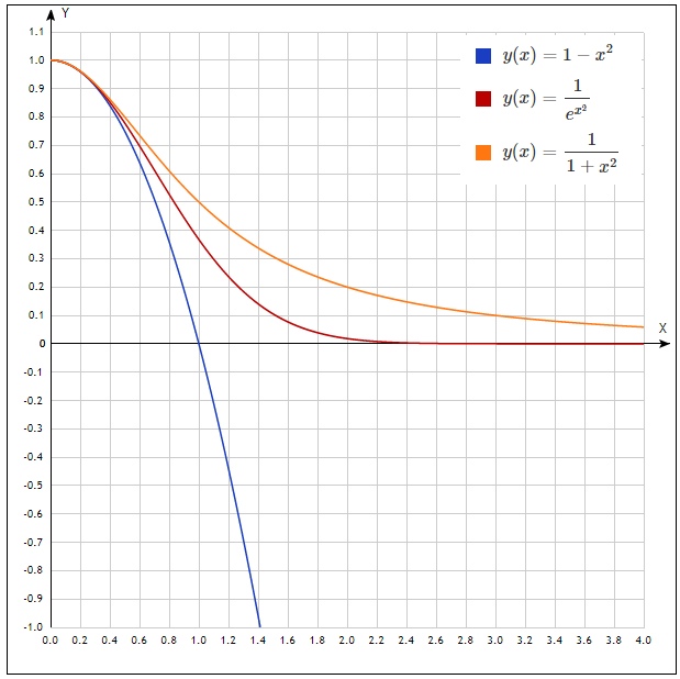
$$t = \ pm x ^ 2 \ to \ left \ {\ begin {array} {l} 0 <\ left ({1 - x ^ 2} \ right) e ^ {x ^ 2} <1 \\ 0 < \ left ({1 + x ^ 2} \ right) e ^ {- x ^ 2} <1 \\ \ end {array} \ right. \ to \ left \ {\ begin {array} {l} 0 <\ left ({1 - x ^ 2} \ right) <e ^ {- x ^ 2} \\ 0 <e ^ {- x ^ 2} <\ frac {1} {{1 + x ^ 2}} \\ \ end {array} \ right.$$

In the first inequality, we restrict the variation (0.1), and in the second, the interval (0; + ∞), we raise both inequalities to the power n, since inequalities with positive terms can be raised to any positive degree. We get:

$$

$$\ begin {array} {* {20} c} {\ left \ {\ begin {array} {l} \ left ({1 - x ^ 2} \ right) ^ n <e ^ {- nx ^ 2} \\ 0 <x <1 \\ \ end {array} \ right.} & {\ Left \ {\ begin {array} {l} e ^ {- nx ^ 2} <\ frac {1} {{\ left ({1 + x ^ 2} \ right) ^ n}} \\ x> 1 \\ \ end {array} \ right.} \\ \ end {array}$$

Let us construct graphs for n = 1 to demonstrate the inequalities



Now we try to integrate the inequalities within the limits indicated in the corresponding systems. And immediately combine everything into one inequality:

$$

$$\ int \ limits_0 ^ 1 {\ left ({1 - x ^ 2} \ right) ^ n dx} <\ int \ limits_0 ^ 1 {e ^ {- nx ^ 2} dx} <\ int \ limits_0 ^ \ infty {e ^ {- nx ^ 2} dx} <\ int \ limits_0 ^ \ infty {\ frac {1} {{\ left ({1 + x ^ 2} \ right) ^ n}} dx}$$

Again, if you look at the graphs, then this inequality is true.



Given a small replacement, it is easy to see that:

$$

$$\ int \ limits_0 ^ \ infty {e ^ {- nx ^ 2} dx} = \ left [\ begin {array} {l} p = \ sqrt nx \\ p ^ 2 = nx ^ 2 \\ \ frac { {dp}} {{\ sqrt n}} = dx \\ \ end {array} \ right] = \ frac {1} {{\ sqrt n}} \ int \ limits_0 ^ \ infty {e ^ {- p ^ 2} dp} = \ frac {1} {{\ sqrt n}} I$$

Those. in that large inequality in the middle, we have the Euler-Poisson integral, and now we need to find the integrals that stand at the borders of this inequality.



Find the integral from the left border:

$$

$$\ begin {array} {l} \ int \ limits_0 ^ 1 {\ left ({1 - x ^ 2} \ right) ^ n dx} = \ left [{\ begin {array} {* {20} c} \ begin {array} {l} x = \ sin t \\ dx = \ cos tdt \\ 1 - x ^ 2 = 1 - \ sin ^ 2 t = \ cos ^ 2 t \\ \ end {array} & \ begin {array} {l} x = 1 \ to t = \ arcsin 1 = \ frac {\ pi} {2} \\ x = 0 \ to t = \ arcsin 0 = 0 \\ \ end {array} \\ \ end {array}} \ right] = \\ = \ int \ limits_0 ^ {\ frac {\ pi} {2}} {\ cos ^ {2n} t \ cdot \ cos tdt} = \ int \ limits_0 ^ { \ frac {\ pi} {2}} {\ cos ^ {2n + 1} tdt} \\ \ end {array}$$

In order to calculate and evaluate it, let's first find a general integral. Now I will show you how to derive the reduction formula (in mathematics, such formulas mean lowering the degree) for a given integral.

$$

$$\ begin {array} {l} \ int \ limits_ \ alpha ^ \ beta {\ cos ^ n tdt} = \ int \ limits_ \ alpha ^ \ beta {\ cos ^ {n - 1} t \ cos tdt} = \ int \ limits_ \ alpha ^ \ beta {\ cos ^ {n - 1} t \ cdot d \ left ({\ sin t} \ right)} = \\ = \ left [{\ begin {array} {* { 20} c} {u = \ cos ^ {n - 1} t} & {du = - \ left ({n - 1} \ right) \ cos ^ {n - 2} t \ sin tdt} \\ {dv = d \ left ({\ sin t} \ right)} & {v = \ sin t} \\ \ end {array}} \ right] = \\ = \ left. {\ cos ^ {n - 1} t \ sin t} \ right | _ \ alpha ^ \ beta + \ left ({n - 1} \ right) \ int \ limits_ \ alpha ^ \ beta {\ cos ^ {n - 2} t \ sin ^ 2 tdt} = \\ = \ left. {\ cos ^ {n - 1} t \ sin t} \ right | _ \ alpha ^ \ beta + \ left ({n - 1} \ right) \ int \ limits_ \ alpha ^ \ beta {\ cos ^ {n - 2} t \ left ({1 - \ cos ^ 2 t} \ right) dt} = \\ = \ left. {\ cos ^ {n - 1} t \ sin t} \ right | _ \ alpha ^ \ beta + \ left ({n - 1} \ right) \ int \ limits_ \ alpha ^ \ beta {\ cos ^ {n - 2} tdt} - \ left ({n - 1} \ right) \ int \ limits_ \ alpha ^ \ beta {\ cos ^ n tdt} \\ \ end {array}$$

$$

$$\ begin {array} {l} \ int \ limits_ \ alpha ^ \ beta {\ cos ^ n tdt} = \ left. {\ cos ^ {n - 1} t \ sin t} \ right | _ \ alpha ^ \ beta + \ left ({n - 1} \ right) \ int \ limits_ \ alpha ^ \ beta {\ cos ^ {n - 2} tdt} - \ left ({n - 1} \ right) \ int \ limits_ \ alpha ^ \ beta {\ cos ^ n tdt} \\ \ int \ limits_ \ alpha ^ \ beta {\ cos ^ n tdt } + \ left ({n - 1} \ right) \ int \ limits_ \ alpha ^ \ beta {\ cos ^ n tdt} = \ left. {\ cos ^ {n - 1} t \ sin t} \ right | _ \ alpha ^ \ beta + \ left ({n - 1} \ right) \ int \ limits_ \ alpha ^ \ beta {\ cos ^ {n - 2} tdt} \\ n \ int \ limits_ \ alpha ^ \ beta {\ cos ^ n tdt = \ left. {\ cos ^ {n - 1} t \ sin t} \ right | _ \ alpha ^ \ beta + \ left ({n - 1} \ right) \ int \ limits_ \ alpha ^ \ beta {\ cos ^ {n - 2} tdt}} \\ \ int \ limits_ \ alpha ^ \ beta {\ cos ^ n tdt = \ frac {1} {n} \ left. {\ cos ^ {n - 1} t \ sin t} \ right | _ \ alpha ^ \ beta + \ frac {{n - 1}} {n} \ int \ limits_ \ alpha ^ \ beta {\ cos ^ { n - 2} tdt}} \\ \ end {array}$$

Now, if using the reduction formula we consider the same integral, but with our limits from 0 to π / 2, then we can make some simplifications:

$$

$$\ begin {array} {l} \ int \ limits_0 ^ {\ frac {\ pi} {2}} {\ cos ^ n tdt = \ frac {1} {n} \ left. {\ cos ^ {n - 1} t \ sin t} \ right | _0 ^ {\ frac {\ pi} {2}} + \ frac {{n - 1}} {n} \ int \ limits_0 ^ {\ frac {\ pi} {2}} {\ cos ^ {n - 2} tdt}} = \ left [{\ frac {1} {n} \ left. {\ cos ^ {n - 1} t \ sin t} \ right | _0 ^ {\ frac {\ pi} {2}} = 0} \ right] = \\ = \ frac {{n - 1}} { n} \ int \ limits_0 ^ {\ frac {\ pi} {2}} {\ cos ^ {n - 2} tdt} = \ frac {{n - 1}} {n} \ left ({\ frac {1 } {{n - 2}} \ left. {\ cos ^ {n - 3} t \ sin t} \ right | _0 ^ {\ frac {\ pi} {2}} + \ frac {{n - 3} } {{n - 2}} \ int \ limits_0 ^ {\ frac {\ pi} {2}} {\ cos ^ {n - 4} tdt}} \ right) = \\ = \ frac {{n - 1 }} {n} \ left ({\ frac {{n - 3}} {{n - 2}} \ int \ limits_0 ^ {\ frac {\ pi} {2}} {\ cos ^ {n - 4} tdt}} \ right) = \ frac {{n - 1}} {n} \ left ({\ frac {{n - 3}} {{n - 2}} \ left ({\ frac {{n - 5 }} {{n - 4}} \ int \ limits_0 ^ {\ frac {\ pi} {2}} {\ cos ^ {n - 6} tdt}} \ right)} \ right) = \\ = \ frac {{n - 1}} {n} \ left ({\ frac {{n - 3}} {{n - 2}} \ left ({\ frac {{n - 5}} {{n - 4}} \ left ({\ frac {{n - 7}} {{n - 6}} \ int \ limits_0 ^ {\ frac {\ pi} {2}} {\ cos ^ {n - 8} tdt}} \ right )} \ right)} \ right) = ... \\ \ end {array}$$

As we see, you can lower it to infinity (depends on n). However, there is one subtlety. The formula changes depending on whether n is an even number or not.

For this, we consider two cases.

$$

$$\ begin {array} {l} n = 10: \\ \ int \ limits_0 ^ {\ frac {\ pi} {2}} {\ cos ^ {10} tdt} = \ frac {{9 \ cdot 7 \ cdot 5 \ cdot 3}} {{10 \ cdot 8 \ cdot 6 \ cdot 4}} \ int \ limits_0 ^ {\ frac {\ pi} {2}} {\ cos ^ 2 tdt} = \ frac {{9 \ cdot 7 \ cdot 5 \ cdot 3}} {{10 \ cdot 8 \ cdot 6 \ cdot 4}} \ int \ limits_0 ^ {\ frac {\ pi} {2}} {\ left ({\ frac {1 } {2} + \ frac {1} {2} \ cos 2t} \ right) dt} = \\ = \ frac {{9 \ cdot 7 \ cdot 5 \ cdot 3}} {{10 \ cdot 8 \ cdot 6 \ cdot 4}} \ left. {\ left ({\ frac {1} {2} t + \ frac {1} {2} \ sin 2t} \ right)} \ right | _0 ^ {\ frac {\ pi} {2}} = \ frac {{9 \ cdot 7 \ cdot 5 \ cdot 3}} {{10 \ cdot 8 \ cdot 6 \ cdot 4}} \ cdot \ frac {\ pi} {4} = \ frac {{9 \ cdot 7 \ cdot 5 \ cdot 3 \ cdot 1}} {{10 \ cdot 8 \ cdot 6 \ cdot 4 \ cdot 2}} \ cdot \ frac {\ pi} {2} = \\ = \ frac {{\ left ({n - 1} \ right) !!}} {{n !!}} \ cdot \ frac {\ pi} {2} \\ \ end {array}$$

$$

$$\ begin {array} {l} n = 9: \\ \ int \ limits_0 ^ {\ frac {\ pi} {2}} {\ cos ^ 9 tdt} = \ frac {{8 \ cdot 6 \ cdot 4 \ cdot 2}} {{9 \ cdot 7 \ cdot 5 \ cdot 3}} \ int \ limits_0 ^ {\ frac {\ pi} {2}} {\ cos tdt} = \ frac {{8 \ cdot 6 \ cdot 4 \ cdot 2}} {{9 \ cdot 7 \ cdot 5 \ cdot 3}} left. {\ left ({\ sint} \ right)} \ right | _0 ^ {\ frac {\ pi} {2}} = \\ = \ frac {{8 \ cdot 6 \ cdot 4 \ cdot 2}} { {9 \ cdot 7 \ cdot 5 \ cdot 3 \ cdot 1}} = \ frac {{\ left ({n - 1} \ right) !!}} {{n !!}} \\ \ end {array}$$

Where is n !! - double factorial. The double factorial of n is denoted by n !! and is defined as the product of all natural numbers in the interval [1, n] having the same parity as n



Due to the fact that 2n + 1 is an odd number for any value of n, we obtain for the left boundary of our inequality:

$$

$$\ int \ limits_0 ^ {\ frac {\ pi} {2}} {\ cos ^ {2n + 1} tdt} = \ frac {{\ left ({2n} \ right) !!}} {{\ left ({2n + 1} \ right) !!}}$$

Find the integral from the right border:

(here we use the same reduction formula that was proved earlier)

$$

$$\ begin {array} {l} \ int \ limits_0 ^ \ infty {\ frac {1} {{\ left ({1 + x ^ 2} \ right) ^ n}} dx = \ left [\ begin {array } {l} x = \ tan t \ to \ begin {array} {* {20} c} {x = 0 \ to t = 0} \\ {x = \ infty \ to t = \ frac {\ pi} {2}} \\ \ end {array} \\ dx = \ frac {{dt}} {{\ cos ^ 2 t}} \\ \ frac {1} {{1 + x ^ 2}} = \ frac {1} {{1 + \ tan ^ 2 t}} = \ cos ^ 2 t \\ \ end {array} \ right]} = \\ = \ int \ limits_0 ^ {\ frac {\ pi} {2} } {\ cos ^ {2n - 2} tdt} = \ left [{\ left ({2n - 2} \ right) - {\ rm {even}}} right] = \ frac {{\ left ({2n - 3} \ right) !!}} {{\ left ({2n - 2} \ right) !!}} \ cdot \ frac {\ pi} {2} \\ \ end {array}$$

After we have estimated the left and right sides of the inequality, we make some transformations to evaluate the limits of the left and right sides of the inequality, provided that n tends to ∞:

$$

$$\ begin {array} {l} \ frac {{\ left ({2n} \ right) !!}} {{\ left ({2n + 1} \ right) !!}} <\ frac {1} { {\ sqrt n}} \ cdot I <\ frac {{\ left ({2n - 3} \ right) !!}} {{\ left ({2n - 2} \ right) !!}} \ cdot \ frac {\ pi} {2} \\ \ sqrt n \ cdot \ frac {{\ left ({2n} \ right) !!}} {{\ left ({2n + 1} \ right) !!}} <I <\ sqrt n \ cdot \ frac {{\ left ({2n - 3} \ right) !!}} {{\ left ({2n - 2} \ right) !!}} \ cdot \ frac {\ pi} {2} \\ \ end {array}$$

Square both sides of the inequality:

$$

$$n \ cdot \ frac {{\ left ({\ left ({2n} \ right) !!} \ right) ^ 2}} {{\ left ({\ left ({2n + 1} \ right) !! } \ right) ^ 2}} <I ^ 2 <n \ cdot \ frac {{\ left ({\ left ({2n - 3} \ right) !!} \ right) ^ 2}} {{\ left ( {\ left ({2n - 2} \ right) !!} \ right) ^ 2}} \ cdot \ frac {{\ pi ^ 2}} {4}$$

Now let's do a little digression. In 1655, John Wallis (an English mathematician, one of the forerunners of mathematical analysis.) Proposed a formula for determining the number π. J. Wallis came to her, calculating the area of ​​a circle. This product converges extremely slowly; therefore, the Wallis formula is of little use for practical calculation of the number π. But it’s great for evaluating our expression :)

$$

$$\ pi = \ mathop {\ lim} \ limits_ {n \ to \ infty} \ frac {1} {n} \ left [{\ frac {{\ left ({2n} \ right) !!}} {{ \ left ({2n - 1} \ right) !!}}} \ right] ^ 2$$

Now we transform our inequality so that we can see where to substitute the Wallis formula:

$$

$$\ begin {array} {l} \ frac {{n ^ 2}} {{\ left ({2n + 1} \ right) ^ 2}} \ cdot \ frac {1} {n} \ cdot \ frac { {\ left ({\ left ({2n} \ right) !!} \ right) ^ 2}} {{\ left ({\ left ({2n - 1} \ right) !!} \ right) ^ 2} } <I ^ 2 <\ frac {1} {{\ frac {1} {n} \ cdot \ frac {{\ left ({\ left ({2n - 2} \ right) !!} \ right) ^ 2 }} {{\ left ({\ left ({2n - 3} \ right) !!} \ right) ^ 2}}}} \ cdot \ frac {{\ pi ^ 2}} {4} \\ \ mathop {\ lim} \ limits_ {n \ to \ infty} \ left [{\ frac {{n ^ 2}} {{\ left ({2n + 1} \ right) ^ 2}}} \ right] \ cdot \ mathop {\ lim} \ limits_ {n \ to \ infty} \ left [{\ frac {1} {n} \ cdot \ frac {{\ left ({\ left ({2n} \ right) !!} \ right ) ^ 2}} {{\ left ({\ left ({2n - 1} \ right) !!} \ right) ^ 2}}} \ right] <I ^ 2 <\ frac {1} {{\ mathop {\ lim} \ limits_ {n \ to \ infty} \ left [{\ frac {1} {n} \ cdot \ frac {{\ left ({\ left ({2n - 2} \ right) !!} \ right) ^ 2}} {{\ left ({\ left ({2n - 3} \ right) !!} \ right) ^ 2}}} \ right]}} \ cdot \ frac {{\ pi ^ 2} } {4} \\ \ frac {1} {4} \ cdot \ pi <I ^ 2 <\ frac {1} {\ pi} \ cdot \ frac {{\ pi ^ 2}} {4} \ to \ frac {\ pi} {4} <I ^ 2 <\ frac {\ pi} {4} \\ I ^ 2 = \ frac {\ pi} {4} \ to I = \ frac {{\ sqrt \ pi}} {2} \\ \ end {array}$$

It follows from the Wallis formula that both the left and right expressions tend to π / 4 as n → ∞

Due to the fact that the function exp [-x²] is even, we safely assume that

$$

$$\ int \ limits_ {- \ infty} ^ \ infty {e ^ {- x ^ 2} dx} = 2 \ int \ limits_0 ^ \ infty {e ^ {- x ^ 2} dx} = 2 \ cdot \ frac {{\ sqrt \ pi}} {2} = \ sqrt \ pi$$

For the first time, the one-dimensional Gaussian integral was calculated in 1729 by Euler, then Poisson found a simple way to calculate it. In this regard, he received the name of the Euler – Poisson integral.



Let's try to calculate the Gaussian integral. It can be written in different forms. After all, nothing changes the name of the variable by which the integration is taking place.

$$

$$\ begin {array} {l} I = \ int \ limits_0 ^ \ infty {e ^ {- x ^ 2} dx} \\ I = \ int \ limits_ {- \ infty} ^ \ infty {e ^ {- x ^ 2} dx} = \ int \ limits_ {- \ infty} ^ \ infty {e ^ {- y ^ 2} dy} = \ int \ limits_ {- \ infty} ^ \ infty {e ^ {- z ^ 2} dz} \\ \ end {array}$$

You can go from three-dimensional Cartesian to spherical coordinates and consider the cube of the Gaussian integral.

$$

$$\ left \ {\ begin {array} {l} x = r \ sin \ theta \ cos \ varphi \\ y = r \ sin \ theta \ sin \ varphi \\ z = r \ cos \ theta \\ \ end {array} \ right. \ to x ^ 2 + y ^ 2 + z ^ 2 = r ^ 2$$

The Jacobian of this transformation can be calculated as follows:

$$

$$\ begin {array} {l} J = \ left | {\ begin {array} {* {20} c} {\ frac {{\ partial x}} {{\ partial r}}} & {\ frac {{\ partial x}} {{\ partial \ theta}} } & {\ frac {{\ partial x}} {{\ partial \ varphi}}} \\ {\ frac {{\ partial y}} {{\ partial r}}} & {\ frac {{\ partial y }} {{\ partial \ theta}}} & {\ frac {{\ partial y}} {{\ partial \ varphi}}} \\ {\ frac {{\ partial z}} {{\ partial r}} } & {\ frac {{\ partial z}} {{\ partial \ theta}}} & {\ frac {{\ partial z}} {{\ partial \ varphi}}} \\ \ end {array}} \ right | = \ left | {\ begin {array} {* {20} c} {\ sin \ theta \ cos \ varphi} & {r \ cos \ theta \ cos \ varphi} & {- r \ sin \ theta \ sin \ varphi} \\ {\ sin \ theta \ sin \ varphi} & {r \ cos \ theta \ sin \ varphi} & {r \ sin \ theta \ cos \ varphi} \\ {r \ cos \ theta} & {- r \ sin \ theta} & 0 \\ \ end {array}} \ right | = \\ = r ^ 2 \ sin \ theta \\ \ end {array}$$

$$

$$\ begin {array} {l} I ^ 3 = \ int \ limits_ {- \ infty} ^ \ infty {\ int \ limits_ {- \ infty} ^ \ infty {\ int \ limits_ {- \ infty} ^ \ infty {e ^ {- x ^ 2 - y ^ 2 - z ^ 2}} dxdydz}} = \ int \ limits_0 ^ {2 \ pi} {\ int \ limits_0 ^ \ pi {\ int \ limits_0 ^ \ infty { e ^ {- r ^ 2} Jdrd \ theta d} \ varphi =}} \\ = \ int \ limits_0 ^ {2 \ pi} {d \ varphi} \ int \ limits_0 ^ \ pi {\ sin \ theta d \ theta} \ int \ limits_0 ^ \ infty {e ^ {- r ^ 2} r ^ 2 dr} \\ \ end {array}$$

We calculate the integrals sequentially, starting with the inner one.

$$

$$\ begin {array} {l} \ int \ limits_0 ^ \ infty {e ^ {- r ^ 2} r ^ 2 dr} = \ left [\ begin {array} {l} u = r \ to du = dr \\ dv = re ^ {- r ^ 2} dr \ to v = \ int {re ^ {- r ^ 2} dr} = \ frac {1} {2} \ int {e ^ {- r ^ 2} dr ^ 2} = - \ frac {1} {2} e ^ {- r ^ 2} \\ \ end {array} \ right] = \\ = \ left. {\ left ({- \ frac {1} {2} re ^ {- r ^ 2}} \ right)} \ right | _0 ^ \ infty + \ frac {1} {2} \ int \ limits_0 ^ \ infty {e ^ {- r ^ 2} dr} = \ frac {1} {2} \ int \ limits_0 ^ \ infty {e ^ {- r ^ 2} dr} = \ frac {1} {2} \ cdot \ frac {I} {2} = \ frac {I} {4} \\ \ int \ limits_0 ^ \ pi {\ sin \ theta d \ theta} = \ left. {\ left ({- \ cos \ theta} \ right)} \ right | _0 ^ \ pi = \ left ({- \ cos \ pi} \ right) - \ left ({- \ cos 0} \ right) = 1 + 1 = 2 \\ \ int \ limits_0 ^ {2 \ pi} {d \ varphi} = \ left. \ varphi \ right | _0 ^ {2 \ pi} = 2 \ pi \\ \ end {array}$$

Then as a result we get:

$$

$$\ begin {array} {l} I ^ 3 = 2 \ pi \ cdot 2 \ cdot \ frac {I} {4} \ to I ^ 3 = \ pi I \ to I ^ 2 = \ pi \ to I = \ sqrt \ pi \\ I = \ int \ limits_ {- \ infty} ^ \ infty {e ^ {- x ^ 2} dx} = \ sqrt \ pi \\ \ end {array}$$

The Euler-Poisson integral is often used in probability theory.



I hope that for someone the article will be useful and help to understand some mathematical techniques :)