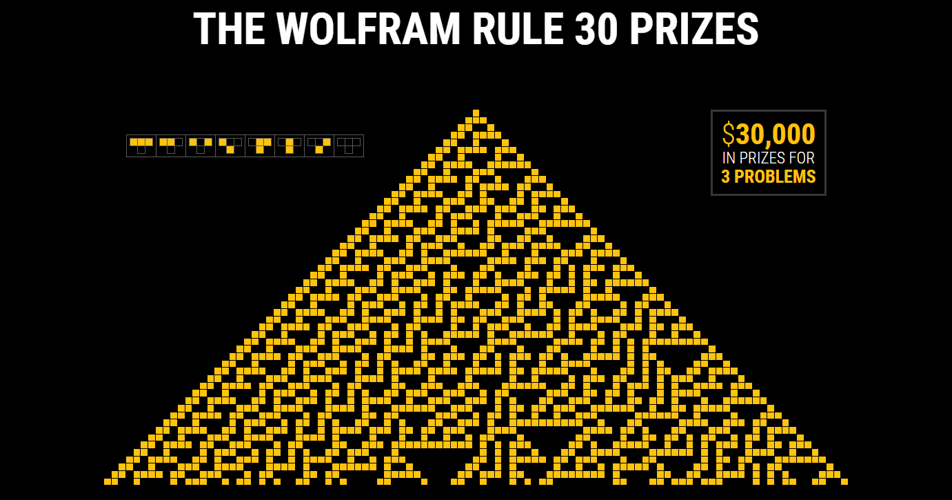
$ 30,000 for solving the problems of Rule 30 for cellular automata - a competition from Stephen Wolfram

Original translation in my blog





Contest website

Let us explain to readers what “Rule 30” means - this is an elementary cellular automaton (see Wiki ), whose state (the rule for constructing a new level of cells based on the old one) in the binary number system is set as 0-0-0-1-1-1 -1-0, which can be interpreted as 30 in decimal notation.

So where did it all start? - “Rule 30”

How can it be that something incredibly simple produces something incredibly complex ? It's been almost 40 years since I first got acquainted with Rule 30, but it still amazes me and delights me. For a long time it became my personal favorite discovery in the history of science, over the years it has changed my whole worldview and led me to a variety of new types of understanding of science, technology, philosophy and much more .



But even after so many years, there are still many basic concepts about Rule 30 that remain inaccessible to us. And so I decided that it was time to do everything possible to stimulate the process of identifying the basic set of these basic patterns.



So, today I am offering applicants $ 30,000 as a total prize for answering the three main questions about Rule 30.



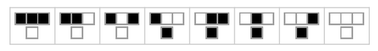
Rule 30 is extremely simple:

There is a sequence of rows of black and white cells (cells) and, given a specific row of black and white cells, the colors of the cells in the row below are determined, considering each cell individually and its adjacent adjacent cells, then the following simple substitution rule is applied to them, namely:

The code

RulePlot[CellularAutomaton[30]]

[Watch the video, which in a couple of minutes tells the essence of cellular automata and Rule 30 - note by the translator]



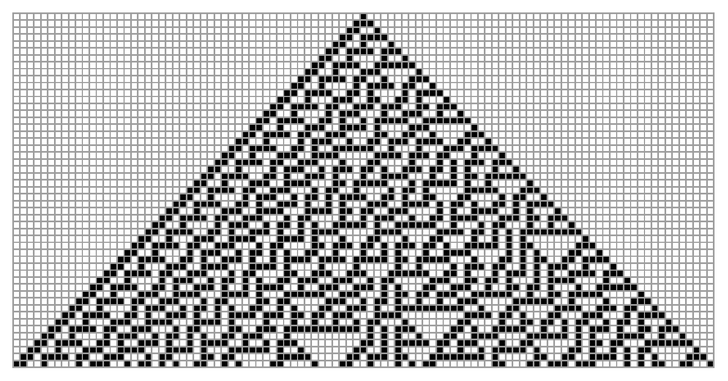
What happens if you start with one black cell? [A row of white cells is taken, infinite on both sides and one black square, then the rules shown above apply to this row, a new row is obtained, etc. - translator’s note ] Suppose (as I myself did at first) that the rule is quite simple, and the template that is obtained on the basis of its work should be accordingly simple too. However, if you conduct an experiment, you will see what happens after the first 50 steps of the algorithm:





Naturally, we can assume that as a result of the algorithm, a much simpler mathematical object will be obtained. However, here's what happens after the first 300 steps:







This shows that there is a certain pattern - on the left side of the pyramid . But at the same time, many aspects of this template look like something formed randomly .



It is incomprehensible that such a simple rule can ultimately lead to such complex system behavior. Based on this, I came to the conclusion that in the computing universe of all possible computer programs, such behavior is quite common, even more so is found almost everywhere.



Based on this hypothesis, I developed an approach to the formation of a completely new type of science - based on the principles of observing the operation of simple algorithms.



Gradually, more evidence was accumulating of these principles.



However, let us return to Rule 30 and consider in detail what exactly it allows us to do, and what is its use? What exactly can be said about the behavior of this algorithm? It is immediately evident that even the answers to the most obvious questions turn out to be difficult.



Even after decades for which no answers were found, I decided that it was time to ask some specific questions about Rule 30, while stimulating this area with serious cash prizes.



I already tried to do something similar in 2007, setting a prize for answering the main question about a specific Turing machine . And in this case, the result was positive and did not take long to wait. Just a few months later this prize was won - having established forever what the simplest of the possible universal Turing machines is, and also very convincingly proving the general principle of computational equivalence , which I personally developed earlier.



The Rule 30 competition again aims to address a key objective, namely: how complex is the behavior of Rule 30 ? Each of the tasks poses a question in this area in its own way and specifically. Like Rule 30 itself, they are all deceptively simple in their original setting. Nevertheless, the solution to any of them will be a huge achievement, which ultimately will help to illuminate the fundamental principles of the properties of the formation of the computing universe, which go far beyond the specifics of Rule 30.



I have been working on each of these issues for over 35 years . And all this time I tried to find the right idea within the framework of consistent mathematical or computational thinking, with the goal of finally solving at least one of these problems. Now I want to open this process to the entire world community. However, I will be interested to know what can be achieved in resolving these issues, and what methods can be used in this case.

Rule 30 - Tasks to Solve

As for the competitive tasks under Rule 30, I give priority to one of the key features of the algorithm of Rule 30, namely: the obvious randomness of the formation of the cells of its central column . Start with one black cell, then take a look at the sequence of color values ​​of the cells in this column and you will come to the conclusion that they are random:









But in what sense are they "truly random" ? And can this assumption be proved? Each of the tasks in the framework of the competition uses its own randomness criterion, and then asks whether the sequence is random in accordance with this criterion.

Task 1: Does the central column always remain non-periodic?

Consider the beginning of the central column of Rule 30:









It is not difficult to find that the values ​​in this column are not repeated - it is not periodic. But the challenge is whether the central column will ever become periodic at all? By launching Rule 30, we see that the sequence does not become periodic even in the first billion steps . What needs to be done in order to establish and prove this for certain.



Here is the link where the first million and first billion values ​​of this sequence are located ( Wolfram data warehouse ).

Task 2: Is each color of the cell (black or white) on average equally likely in the center column?

This is what we get when we count the number of black and white cells sequentially at more steps in the central column of Rule 30 algorithm:









The results are certainly close to equal for black and white cells. Here the problematic (question of the problem) is the question of whether this relation converges to 1 with an increase in the number of steps in the cycle .

Task 3: Does the calculation of the nth cell of the central column require at least O ( n ) operations?

To find the nth cell in the center column, you can always simply run Rule 30 for n steps, calculating the values ​​of all cells inside the rhombus highlighted in the figure below:









But if you do it directly, it will n ² separate cell updates, therefore, the required computing power increases as O ( n ² ). The question of this problem is whether there exists a more (or the most) fastest method for calculating the value of the nth cell without all intermediate calculations - or, in particular, in less than O ( n ) operations .

The numbers that make up Pi

Rule 30 is a product of the computing universe: a system based on the study of possible simple programs with a new intellectual structure, which is provided by the paradigm of computing. However , the tasks that I defined in the competition for Rule 30 have analogues in mathematics, which have been around for centuries .



Consider the values ​​of the numbers in the number Pi . The behavior of these numbers is similar to the generation of data in the central column of the Rule 30 algorithm. That is, there is a given algorithm for calculating them, and once formulated, they seem almost random for any tasks.









Just to make the analog a little closer, here are the first few digits of Pi in the number system with base 2:









And here are the first few bits in the center column of Rule 30:









For fun, you can convert them to decimal:









Of course, the well-known algorithms for calculating the digits of Pi are much more complicated than the relatively simple rule for generating cells in the central column of Rule 30. So, what do we know about the numbers in Pi?



Firstly, we know that they are not repeated. This was proved back in the 60s of the 18th century, when it was shown that Pi is an irrational number , since the only numbers in which the numbers are repeated are rational numbers. (In 1882, it was also shown that Pi is transcendental , that is, that it cannot be expressed through the roots of polynomials).



So what kind of analogy can be drawn with the formulation of problem 2? Do we know that in the sequence of digits of Pi, different digits occur with the same frequency? To date , more than 100 trillion binary digits have been calculated - and the measured digit frequencies are very close (in the first 40 trillion binary digits of Pi, the ratio of Units to Zeros is approximately 0.99999998064). But when calculating the limit, will the frequencies be exactly the same? Scientists have been asking this question for several centuries, but so far mathematics have not been able to give an answer to it.



For rational numbers, the sequences of digits of which they consist are periodic, and it is easy to determine the relative frequencies of occurrence of these numbers in a number. However, for the sequence of digits of all the other “created by nature (naturally constructed)” numbers, in most cases, practically nothing is known about what the frequencies of the digits included in the number tend to. It would be logical to assume that in fact the digits of the Pi number (as well as the central column of Rule 30) are “ normal ” in the sense that not only each individual digit, but also any block of digits of a given length meet with the same limit frequency. And, as was noted in the works on this subject of the 1930s, it is quite possible to “build a digital construction (model)” of normal numbers. The Chemternoun constant obtained by combining the digits of consecutive integers is an example of the above reasoning (the same can be obtained on the basis of any normal number by combining the values ​​of the functions of consecutive integers):









It should be noted that the point here is that for “naturally constructed” numbers formed by combinations of standard mathematical functions, not a single discovered example is found where any regular sequence of numbers would be found. Naturally, in the end, this provision depends on what is meant by “regularity,” and at some stage the task turns into a kind of digital-analog search for extraterrestrial intelligence . However, there is no evidence that it is not possible, for example, to find some complex combination of square roots that would have a sequence of numbers with some very obvious regularity.



So, finally, consider the analogue of Problem 3 for Pi? Unlike Rule 30, where the obvious way to calculate the elements in a sequence is one step at a time, traditional methods for calculating the digits of Pi include getting the best approximations to Pi as an exact number. With the standard (“bizarre”) series invented by Ramanujan in 1910 and improved by the Chudnovsky brothers in 1989, the first few members of this series give the following approximations:









So how many operations are needed to find the nth digit? The number of terms required in the row is O ( n ). But each condition must be calculated with n- digit accuracy, which requires at least O ( n ) separate computational operations, implying that in general computational workloads will be greater than O ( n ).



Until the 1990s, it was assumed that there was no way to calculate the nth digit of Pi without computing all the previous ones. But in 1995, Simon Pluff discovered that in fact it is possible to calculate, although with some probability, the nth digit without calculating the previous ones. And although one would think that this would make it possible to get the nth digit in less than O ( n ) operations, the fact that you need to perform calculations with an accuracy of n- digits means that at least O ( n ) operations.

Results, analogies and intuition

Task 1: Does the central column always remain non-periodic?

Of the three prizes of the Rule 30 contest, this is the one in which most of the progress in resolving this issue has already been achieved. Since it is still unknown whether the central column of Rule 30 will become periodic, Erica Jen showed in 1986 that no two columns can be periodic. And in fact this is so, and one can also argue in favor of the fact that one column in combination with individual cells in another column cannot be periodic .



The proof of the pair of columns uses a feature of Rule 30. Consider the structure of the rule:









It is possible to simply say that for each triple of cells the rule determines the color of the central cell on it, but for Rule 30, you can also effectively execute the rule to the side: taking into account the cell on the right and above, you can also uniquely determine the color of the cell on the left. This means that if you take two adjacent columns, you can restore the entire template on the left :









However, if the columns had a periodic structure, it would immediately follow that the restored template should also be periodic. So, for example, by construction, at least the initial conditions are definitely not periodic, and therefore both columns cannot be periodic. The same statement is true if the columns are not adjacent, and if all cells in both columns are not known. However, there is no known way to distribute this provision for a single column, such as a central column, and thus it does not solve the first task of the competition under Rule 30.



So what can be used to solve it? If it turns out that the central column is ultimately periodic, you could just calculate it. We know that it is not periodic for the first billions of steps, but we can at least assume that there may be a transition process with trillions of steps, after which it becomes periodic.



Do you think this is believable? Transients occur - and theoretically (as in the classical problem of stopping a Turing machine ) they can even be of arbitrary length. Here we’ll look at some example - found during the search - Rules with 4 possible colors (common code 150898). Suppose we run it 200 steps, and, as you can see, the central column will be completely random:









After 500 steps, the entire template looks completely random:









Here you can see that when approaching the central column, something surprising happens: after 251 steps, the central column seems to be reborn to a fixed value (or at least fixed to the next more than a million steps):









Could the same transition occur in Rule 30? Consider the patterns from Rule 30, and select those where the diagonals on the left have periodicity:









Apparently, there is a border that separates the order to the left of the mess to the right. And, at least for the first 100,000 steps or so, it seems that the border shifts on average by about 0.252 steps to the left at each step - with some random deviations :









But how do we eventually find out at what point these fluctuations will cease to be significant, so much so that they force the order on the left to cross the central column and, perhaps, even make the entire template periodic? Judging by the available data, the assumption seems unlikely, while I can’t say exactly how this can be determined.



This, of course, is precisely the case that illustrates the existence of systems with exceptionally long "transients." Now consider the distribution of primes and calculate LogIntegral [ n ] - PrimePi [ n ]









Yes, there are fluctuations, but in this illustration it looks as if this difference will always be in the positive area. And this, for example, is what Ramanujan was discussing, but in the end it turns out that this is not so . At the beginning, the boundary of where he failed was, for that time, astronomically large ( Skives number 10 ^{10 10 964} ). And although no one has yet found an explicit value of n for which the difference is negative, it is known that up to n = 10 ³¹⁷ it must exist (and ultimately the difference will be negative).



I have formed the opinion that nothing of the kind happens to the central column of Rule 30, but so far we have no evidence that this is impossible, this cannot be argued.



It should be noted that it is possible to make the assumption that although it is fundamentally possible to prove periodicity by revealing regularity in the central column of Rule 30, nothing of the kind can be done for non-periodicity. It is known that there are patterns whose central columns are non-periodic, although they are very regular. The main class of such examples are nested templates. Here, for example, is a very simple illustration from Rule 161, in which the center column has white cells when n = 2 ^k :









And here is a slightly more complex example (from the 2-color Rule 69540422 for two neighbors) , in which the central column is a Thue – Morse sequence - ThueMorse [ n ]:









We can assume that the Thue – Morse sequence is generated by the successive application of the substitution:









It turns out that the nth term in this sequence is set as Mod [ DigitCount [ n , 2, 1], 2] - this object will never be periodic.



Could it be that the central column of Rule 30 can be generated by replacement ? If this is so, then I would be struck by this fact (although there would seem to be natural examples when very complex substitution systems appear ), but again, as long as there is no evidence of this.



It should be noted that all competitive tasks from Rule 30 are considered in the formulation of an algorithm that runs on an infinite number of cells. , n , , ( )? , 2 ⁿ — , , . n =5:









n =5 n =11:









, , , , . , 2 ⁿ ( , , ).



, n 30 , , 2 ⁿ . , ( ):









, , n 2 ^{0.63 n} . , , . , , ? .

2: ?

10000 30:









:









:









, , 1 () 0 (), , , , , , , .



. 10 000 :









, 1? …



, :









, , . 1 , :









, ? . , . , , , , .



, , 30, .



, , k . , 2 ^k . , - , , , , 30 k ( ).



, . , , k =22, 2 ^k , , :









, , . , – , , .



— — , , , , , , 30, , , , , .



30 , , « », , , , , , . , «»: 30, , , , , , , , 30.



, . 30, , - , , , 30, , , - .



. 30 , , . , , 30 - ( ), , , , 30. 200 :









, :









, , , 0 1.



1900- . , , FractionalPart [ hn ] n h . , FractionalPart [ h ⁿ ] h ( ), — FractionalPart [(3/2) ⁿ ] — . (, , 16- , , 2- FractionalPart [16 x _{n -1} + r [ n ]], r [ n ] n .)

3: n- O( n ) ?

, 150 :









, ( ), , :









n- ? , , : Mod [ IntegerExponent [ n , 2], 2]. , n , , .



, « »? , n , Log [2, n ] . , , O(log n ) .



- 30? , n- , 30 n ² , , . , -, , , — , , , , , .



« » (, , . .), , , , , (, , 3D- . .), .



, 1980- , , , , , , , .



, 3 30 , , . ( O( n ) ; O( n ^α ) α <2, , , O(log ^β ( n )) — , , .)



3 , , n- , O( n ), 150 .



O ( n )? () , « »? , — — , , .



, . , , , n , , , n , (, «», O(log n ) .



, . , , , , Wolfram Language . « ». , , Wolfram Language , .



, 30 , 3 , , , , , , n- , O( n ) , .



, , . , , . , , , , , — , O(log n ) , n .



, P NP . , 30 ( P LOGTIME ), , , , . , , , n n , O( n ² ) , , P (« »), , , , , NP. («») , , , , 2 ⁿ .



, 2 ⁿ , , . , NP- , , , NP . 30 NP-? , , ( - , 30 NP).



30 . : 30 , , 30, «» , , , , .



, 256 110 ( , ), 110 , , , . , , , «» 110 .









30, , — , «» , . , , 30 , , , , .



, , , , , 30. , , (, ) , , . , , — , . , .



, , 3. , , , , n- ?



, 30 . , 2 ^{m 2} m × m , , . , , , O( n ² ) ( ). , O( n ) ? .



, 1 , , - O( n ) — , « ». , ( , 2 ), , , .



- , , , ? , , .



. «» , , , . 30 - . ( — — 30 Wolfram Language, « !» ).



: « - , , ». ? , , , - . . , — , . , , , — - «» 30.



, 30. , 30 - . , , , - 30 , , , , — 30, , , , .



. , 3 2 6 :









, 6 . ( 2 ). , , .



s- n . s- 3 ⁿ , «» ( b — , 2 6) Mod [ Quotient [3 ⁿ , b ^s ], b]. ? , 3 ⁿ n , : , , 3 ⁿ , log( n ). , , , . , 30, , - , .



3 n - 30 , , O( n ), , n , . , r [ n ] , r [ n ] «O-» n , , MaxLimit [ r [ n ]/ n , n →∞ ]<∞.



, ( - ), . , r [ n ] n , , , - , , r [ n ] . , - n ( - ), r [ n ] . , , , r [ n ] O( n ).

30

, ( , ).



Wolfram Language t 30 :









c [ t ].

1: ?

p i t , t > i , [ t + p ] c [ t ].

2: ?

c [ t ]/ t t →∞ 1/2.

3: n- O( n ) ?

machine[ m ] , m (, TuringMachine [...]), machine[ m ][ n ] { v , t }, v — , t — (, ). :









« m, , machine[ m ] n c [ n ] , n , ». ( m , «» ).

, , , , . 3 ( ), , 1 2, . 3 ( ), , 1 . : 1 , , 3 .



1 , , , , , 2. , 2 - 3. , , O( n ) — , , 3, , .



, , ?



1 , , , 30 - , . , 1 , . , , - , .



( , ), 2, 3 , — , , , . , 3 , , (, , ), O( n ) .



, - . , n n- . . , - , . , , n n . , . , « » . , n , . , , O( n ) .



: ? « », / ( ).



, , ( )? , , , , «» , -, ( ) , .



, , . , , , . , () .



, , , , : « ». , , , .



, — - . - n , . . — (« » . .). , , , .



— , , . , ( FindEquationalProof ). , () .



, , , — , . — , .



, . Wolfram|Alpha (, ) , . , .



, , - , , , , .



? , «» , . Wolfram Language , . Wolfram Language, .



« »? , , - . . - , , «» , , - ( ), . , , «» — , .

?

, ? . . , . - , . . - , , .



, , «» — , — , « ». , 2,3 2007 .



— , , 30, , . . - ( , , ). , , ( ) , , .



n — 30 n , n . Wolfram Language . , 0,4 100 000 :









, 30 Xor [ p , Or [ q , r ]], . , CellularAutomaton :









. . , , 30, , 30 , , , : .



. , , «» . 30 — . , , , .

— , , . , , 30, .



, , 30, . 45° , 30, , . ; . ?



? ? - ? , , , , , .



? 30, . , , , , , . , - , , , , , , - .



– , «» . ( , - ). , , , , « » :









, , , . ? , « » ?



, (, ), , - 30?



« 30». , «» ? 30 , ? «» ?



, , 30, , , , 30, . 256 ( ) , , :









, . , . , , . , , , « 30», .



« 30». 30 ( 1), , — , .



2, 30, , .



3 . n- O( n ^γ ) γ <2 ( - )? , n- , O(log( n )) ? O(log( n )) ? ? . ?



, 30. 30, (, , 110) , 30.



, NP-, 30 , , NP-? , . , , , « », 30?

?

2007 2,3 , — , , , . , . 30? I dont know. 40 , - ( , !). , , (, ) .



, - ( ), , , , , , , . ( ), , , .



, « » ( , ), . , . , (« » . .). . , - « », , , …



, . , , . , , . , .



, 30 40 , - .

Wolfram Language?

« Wolfram » ( ).