Neural network for classifying satellite images using Tensorflow in Python

This is a step-by-step instruction for the classification of multispectral images from the Landsat 5 satellite. Today, in a number of areas, deep learning dominates as a tool for solving complex problems, including geospatial ones. I hope you are familiar with datasets of satellite images, in particular, Landsat 5 TM. If you are a little familiar with machine learning algorithms, this will help you quickly learn this manual. And for those who do not understand, it will be sufficient to know that, in fact, machine learning consists in establishing relationships between several characteristics (a set of attributes X) of an object with its other property (value or label, the target variable Y). We feed the model with many objects for which the characteristics and value of the target indicator / class of the object (labeled data) are known and train it so that it can predict the value of the target variable Y for new data (unmarked).



What is the main problem with satellite imagery?



Two or more classes of objects (for example, buildings, vacant lots and foundation pits) in satellite images can have the same spectral characteristics of the value, therefore, in the last twenty years, their classification has been a difficult task.



Because of this, it is possible to use classic machine learning models with and without a teacher, but their quality will be far from ideal. They always have the same disadvantages. Consider an example:







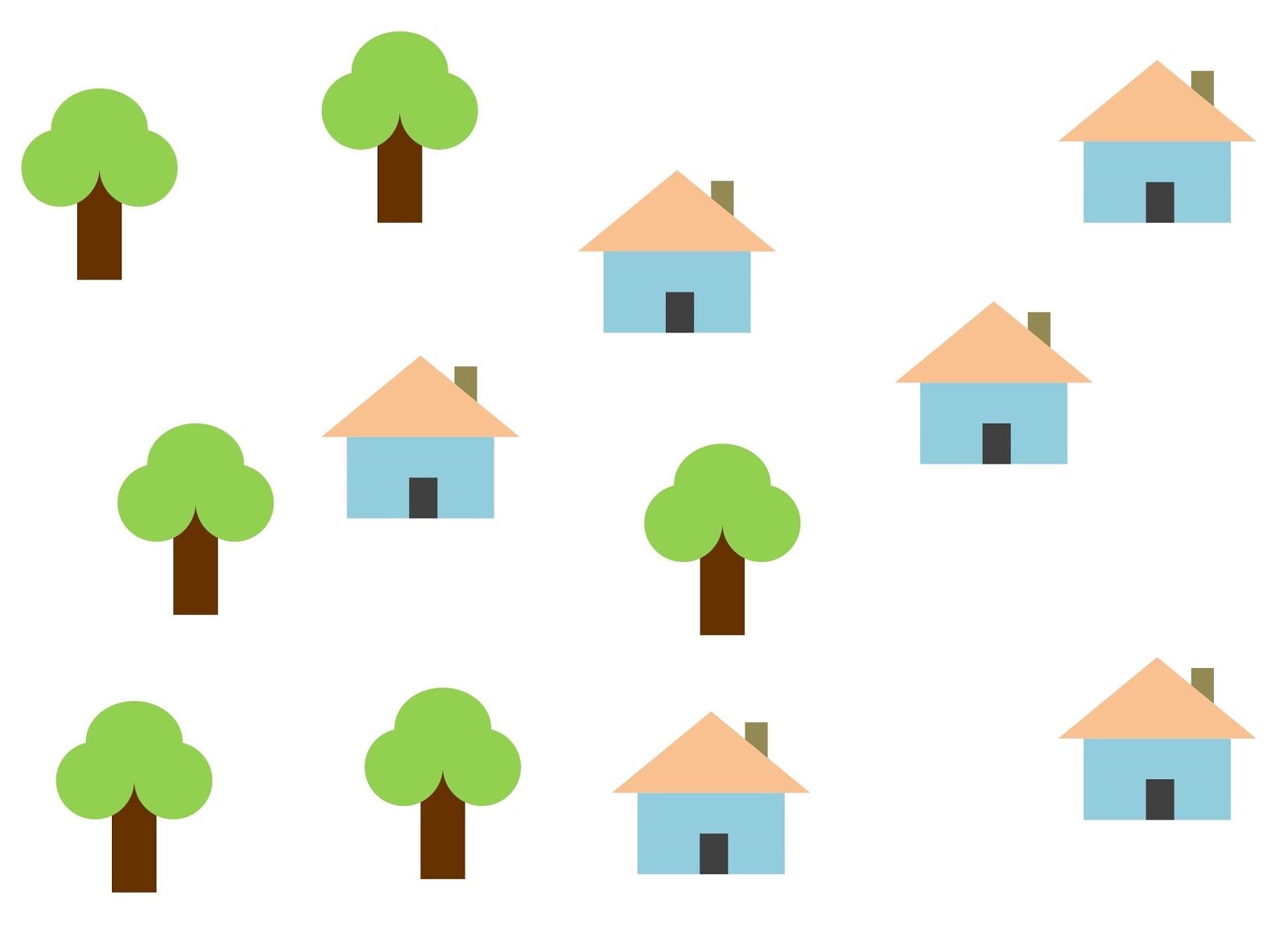
If you use a vertical line as a classifier and move it along the X axis, then classifying images of houses will not be easy. The data is distributed so that it is impossible to separate them into classes using one vertical line (in such cases they say that "objects of different classes are not linearly separable"). But this does not mean that houses cannot be classified at all!







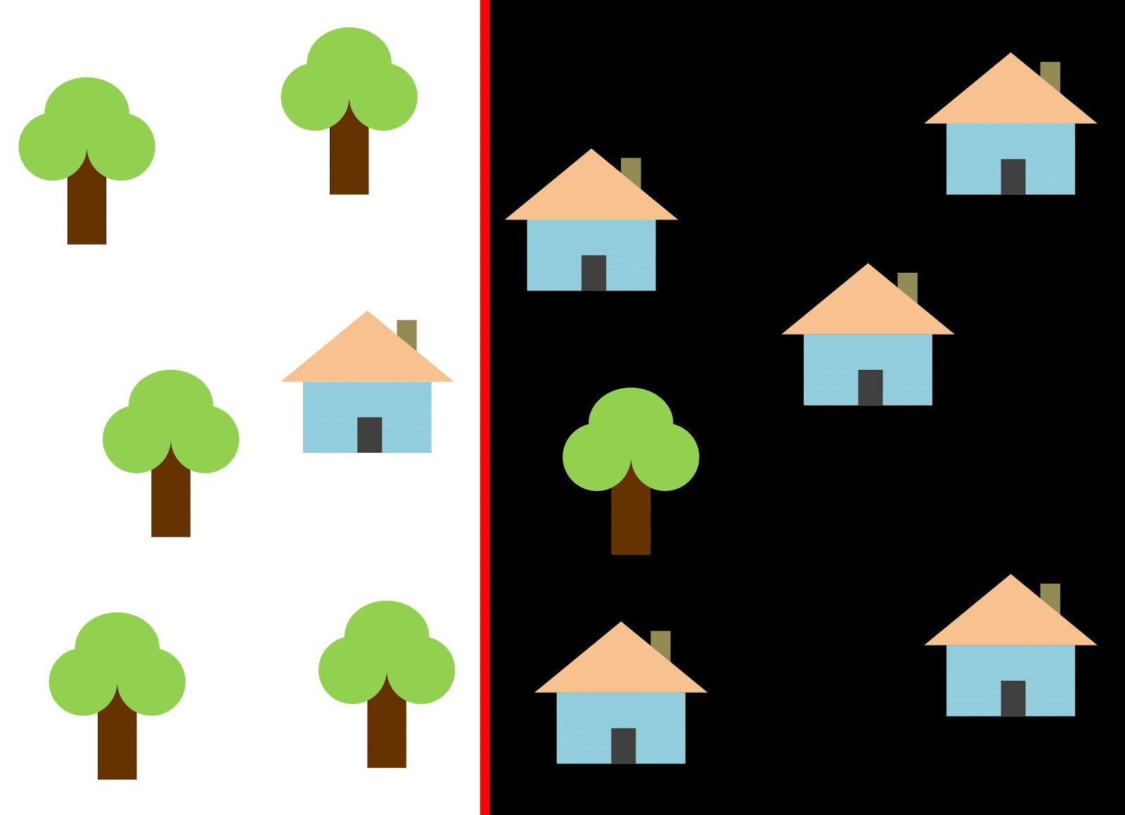
Let's use the red line to separate the two classes. In this case, the classifier identified most of the houses, but one house was not assigned to its class, and three more trees were assigned to the "houses" by mistake. In order not to miss a single house, you can use the classifier in the form of a blue line. Then everything will be covered at home, that is, we say that the recall metric (fullness) is high. However, not all classified values ​​turned out to be houses, that is, we simultaneously got a low value of the precision metric. If we use the green line, then all images classified as houses will really be houses, that is, the classifier will show high accuracy. In this case, the fullness will be less, since the three houses will be unaccounted for. In most cases, we have to find a compromise between accuracy and completeness.



This problem of houses and trees is similar to the problem with buildings, vacant lots and pits. The priority of satellite imagery classification metrics may vary depending on the task. For example, if you need to make sure that all built-up territories are classified as buildings without exception, and you are ready to put up with the presence of pixels of other classes with similar signatures, which will also be classified as buildings, then you need a model with a high completeness. And if it’s more important for you to classify a building, without adding pixels of other classes, and you are ready to abandon the classification of mixed territories, then choose a classifier with high accuracy. In the case of houses and trees, the usual model will use the red line, maintaining a balance between accuracy and completeness.

Data used

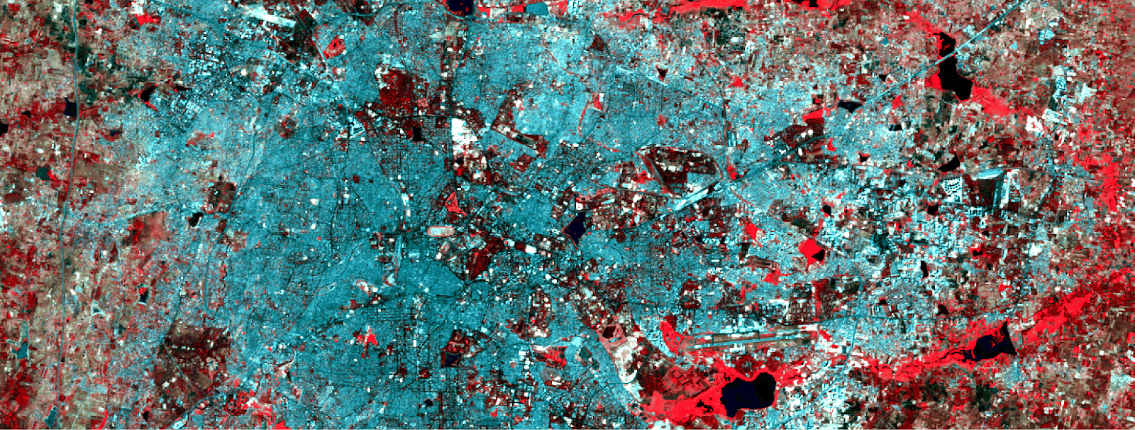
As signs, we will use the values ​​of six ranges (band 2 - band 7) of the image from Landsat 5 TM, and try to predict the binary development class. For training and testing, multispectral data (images and a layer with a binary building class) with Landsat 5 for 2011 for Bangalore will be used. And for prediction will be used multispectral Landsat 5 data obtained in 2005 in Hyderabad.

Since we use tagged data for teaching, this is called teaching with the teacher.







Multispectral training data and the corresponding binary layer with development.



To create a neural network, we will use Python — the Google Tensorflow library. We will also need these libraries:

1. pyrsgis - for reading and writing GeoTIFF.
   
   
2. scikit-learn - for data preprocessing and accuracy assessment.
   
   
3. numpy - for basic operations with arrays.
   
   

And now, without further ado, let's write the code.



Put all three files in a directory, write the path and names of the input files in the script, and then read the GeoTIFF files.

import os from pyrsgis import raster os.chdir("E:\\yourDirectoryName") mxBangalore = 'l5_Bangalore2011_raw.tif' builtupBangalore = 'l5_Bangalore2011_builtup.tif' mxHyderabad = 'l5_Hyderabad2011_raw.tif' # Read the rasters as array ds1, featuresBangalore = raster.read(mxBangalore, bands='all') ds2, labelBangalore = raster.read(builtupBangalore, bands=1) ds3, featuresHyderabad = raster.read(mxHyderabad, bands='all')
      
      

        
        
        
      

    
        
        
        
      
      

        
        
        
      

    
     

The raster



module from the pyrsgis



package reads GeoTIFF geolocation data and digital number (DN) values ​​as separate NumPy arrays. If you are interested in details, read here .



Now we will display the size of the read data.

 print("Bangalore multispectral image shape: ", featuresBangalore.shape) print("Bangalore binary built-up image shape: ", labelBangalore.shape) print("Hyderabad multispectral image shape: ", featuresHyderabad.shape)
      
      

        
        
        
      

    
        
        
        
      
      

        
        
        
      

    
     

Result:

 Bangalore multispectral image shape: 6, 2054, 2044 Bangalore binary built-up image shape: 2054, 2044 Hyderabad multispectral image shape: 6, 1318, 1056
      
      

        
        
        
      

    
        
        
        
      
      

        
        
        
      

    
     

As you can see, the images of Bangalore have the same number of rows and columns as in the binary layer (corresponding to the building). The number of layers in multispectral images in Bangalore and Hyderabad also coincides. The model will learn to decide which pixels belong to the building and which are not, based on the corresponding values ​​for all 6 spectra. Therefore, multispectral images must have the same number of features (ranges) listed in the same order.



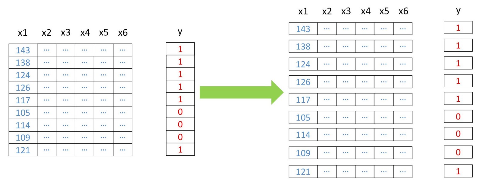
Now we turn the arrays into two-dimensional, where each row represents a separate pixel, because this is necessary for the operation of most machine learning algorithms. We will do this using the convert



module from the pyrsgis



package.





Data restructuring scheme.

 from pyrsgis.convert import changeDimension featuresBangalore = changeDimension(featuresBangalore) labelBangalore = changeDimension (labelBangalore) featuresHyderabad = changeDimension(featuresHyderabad) nBands = featuresBangalore.shape[1] labelBangalore = (labelBangalore == 1).astype(int) print("Bangalore multispectral image shape: ", featuresBangalore.shape) print("Bangalore binary built-up image shape: ", labelBangalore.shape) print("Hyderabad multispectral image shape: ", featuresHyderabad.shape)
      
      

        
        
        
      

    
        
        
        
      
      

        
        
        
      

    
     

Result:

 Bangalore multispectral image shape: 4198376, 6 Bangalore binary built-up image shape: 4198376 Hyderabad multispectral image shape: 1391808, 6
      
      

        
        
        
      

    
        
        
        
      
      

        
        
        
      

    
     

In the seventh row, we extracted all the pixels with a value of 1. This helps to avoid problems with pixels without information (NoData), which often have extremely high or low values.

Now we will divide the data into training and validation samples. This is necessary so that the model does not see the test data and works just as well with the new information. Otherwise, the model will be retrained and will work well only on training data.

 from sklearn.model_selection import train_test_split xTrain, xTest, yTrain, yTest = train_test_split(featuresBangalore, labelBangalore, test_size=0.4, random_state=42) print(xTrain.shape) print(yTrain.shape) print(xTest.shape) print(yTest.shape)
      
      

        
        
        
      

    
        
        
        
      
      

        
        
        
      

    
     

Result:

 (2519025, 6) (2519025,) (1679351, 6) (1679351,) test_size=0.4
      
      

        
        
        
      

    
        
        
        
      
      

        
        
        
      

    
     

means that the data is divided into training and validation in a ratio of 60/40.

Many machine learning algorithms, including neural networks, need normalized data. This means that they must be distributed within a given range (in this case, from 0 to 1). Therefore, to fulfill this requirement, we normalize the symptoms. This can be done by extracting the minimum value and then dividing it by the spread (the difference between the maximum and minimum values). Since the Landsat dataset is eight-bit, the minimum and maximum values ​​will be 0 and 255 (2 ^⁸ = 256 values).



Note that for normalization it is always better to calculate the minimum and maximum values ​​based on the data. To simplify the task, we will adhere to the eight-bit range by default.



Another stage of preliminary processing is the transformation of the matrix of attributes from two-dimensional to three-dimensional, so that the model perceives each row as a separate pixel (a separate learning object).

 # Normalise the data xTrain = xTrain / 255.0 xTest = xTest / 255.0 featuresHyderabad = featuresHyderabad / 255.0 # Reshape the data xTrain = xTrain.reshape((xTrain.shape[0], 1, xTrain.shape[1])) xTest = xTest.reshape((xTest.shape[0], 1, xTest.shape[1])) featuresHyderabad = featuresHyderabad.reshape((featuresHyderabad.shape[0], 1, featuresHyderabad.shape[1])) # Print the shape of reshaped data print(xTrain.shape, xTest.shape, featuresHyderabad.shape)
      
      

        
        
        
      

    
        
        
        
      
      

        
        
        
      

    
     

Result:

 (2519025, 1, 6) (1679351, 1, 6) (1391808, 1, 6)
      
      

        
        
        
      

    
        
        
        
      
      

        
        
        
      

    
     

Everything is ready, let's assemble our model with keras . To get started, let's use the sequential model, adding layers one after another. We will have one input layer with the number of nodes equal to the number of ranges ( nBands



) - in our case there are 6. We will also use one hidden layer with 14 nodes and the ReLu



activation ReLu



. The last layer consists of two nodes for determining the binary building class with the softmax



activation softmax



, which is suitable for displaying a categorized result. Read more about activation functions here .

 from tensorflow import keras # Define the parameters of the model model = keras.Sequential([ keras.layers.Flatten(input_shape=(1, nBands)), keras.layers.Dense(14, activation='relu'), keras.layers.Dense(2, activation='softmax')]) # Define the accuracy metrics and parameters model.compile(optimizer="adam", loss="sparse_categorical_crossentropy", metrics=["accuracy"]) # Run the model model.fit(xTrain, yTrain, epochs=2)
      
      

        
        
        
      

    
        
        
        
      
      

        
        
        
      

    
     

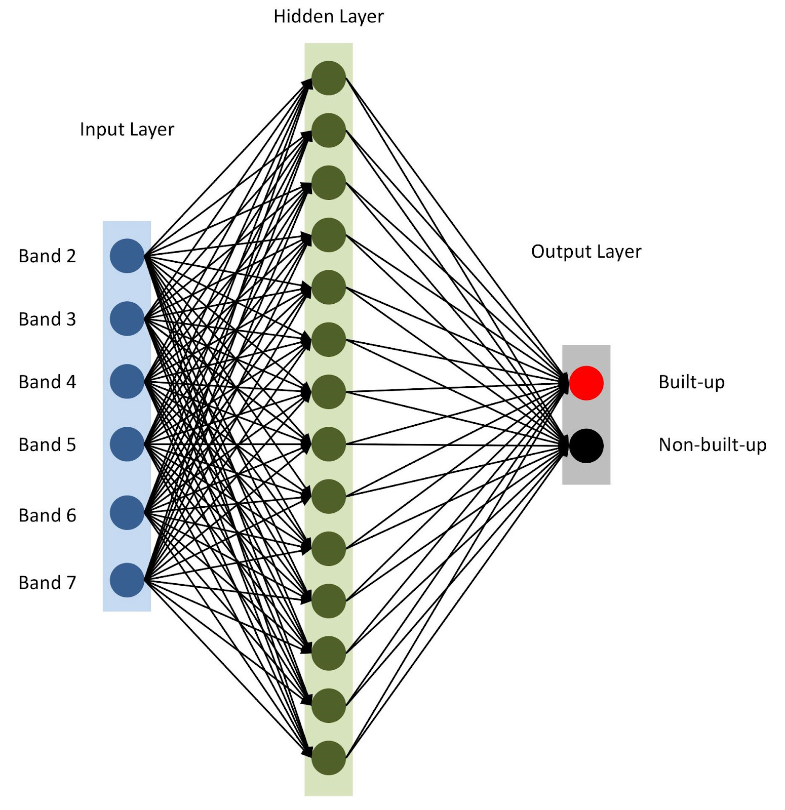
Neural network architecture



As mentioned in line 10, we specify adam



as the model optimizer (there are several others ). In this case, we will use cross entropy as a loss function (en. categorical-sparse-crossentropy



- more about it is written here ). To assess the quality of the model, we will use the accuracy



metric.



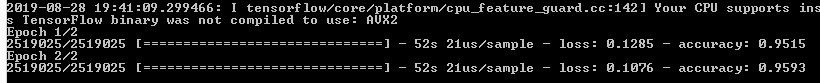
Finally, we will start training our model for two eras (or iterations) on xTrain



and yTrain



. This will take some time, depending on the size of the data and processing power. Here is what you will see after compilation:







Let's predict the values ​​for the validation data that we store separately and calculate various accuracy metrics.

 from sklearn.metrics import confusion_matrix, precision_score, recall_score # Predict for test data yTestPredicted = model.predict(xTest) yTestPredicted = yTestPredicted[:,1] # Calculate and display the error metrics yTestPredicted = (yTestPredicted>0.5).astype(int) cMatrix = confusion_matrix(yTest, yTestPredicted) pScore = precision_score(yTest, yTestPredicted) rScore = recall_score(yTest, yTestPredicted) print("Confusion matrix: for 14 nodes\n", cMatrix) print("\nP-Score: %.3f, R-Score: %.3f" % (pScore, rScore))
      
      

        
        
        
      

    
        
        
        
      
      

        
        
        
      

    
     

The softmax



function generates separate columns for probability values ​​for each class. We use only the values ​​for the first class ("there is a building"), as can be seen from the sixth line of the code above. Evaluating the work of geospatial analysis models is not so simple, unlike other classical machine learning tasks. It will be unfair to rely on a generalized total error. The key to a successful model is spatial layout. Thus, the error matrix (confusion matrix), accuracy and completeness can give a more correct idea of ​​the quality of the model.





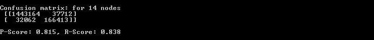
So the console displays the error matrix, accuracy and completeness.



As you can see from the confusion matrix, there are thousands of pixels that are related to buildings, but are classified differently, and vice versa. However, their share of the total data volume is not too large. The accuracy and completeness of the test data exceeded the threshold of 0.8.



You can spend more time and perform several iterations to find the optimal number of hidden layers, the number of nodes in each hidden layer, as well as the number of eras to achieve the desired accuracy. As needed, remote sensing indices such as NDBI or NDWI can be used as features. When achieving the desired accuracy, use the model to predict development based on new data and export the result to GeoTIFF. For such tasks, you can use a similar model with minor changes.

 predicted = model.predict(feature2005) predicted = predicted[:,1] #Export raster prediction = np.reshape(predicted, (ds.RasterYSize, ds.RasterXSize)) outFile = 'Hyderabad_2011_BuiltupNN_predicted.tif' raster.export(prediction, ds3, filename=outFile, dtype='float')
      
      

        
        
        
      

    
        
        
        
      
      

        
        
        
      

    
     

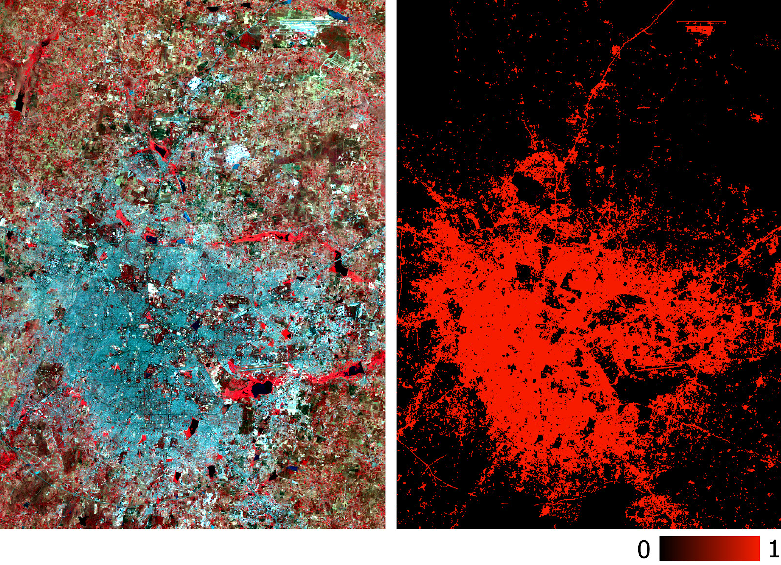
Please note that we export GeoTIFF with predicted probability values, and not with their threshold-binarized version. Later in the GIS environment, we can set the threshold value of a layer of type float, as shown in the figure below.





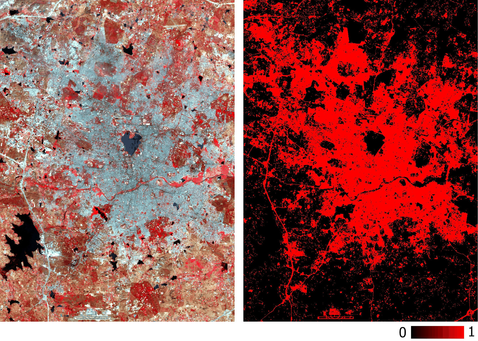
Hyderabad built-up layer predicted by the model based on multispectral data.



Model accuracy has already been measured with precision and recall. You can also carry out traditional checks (for example, using the kappa coefficient) on a new predicted layer. In addition to the aforementioned difficulties with the classification of satellite images, other obvious limitations include the impossibility of forecasting based on images taken at different times of the year and in different regions, since they will have different spectral signatures.



The model described in this article has the simplest architecture for neural networks. Better results can be achieved with more complex models, including convolutional neural networks. The main advantage of such a classification is its scalability (applicability) after training the model.



The data used and all the code are here .