"Technology" of obtaining dynamic equations of TAU. And why is System Identification is sucks, and "honest physics" rules
When discussing the previous article about model-oriented design, a reasonable question arose: if we use the data of the experiment, but is it possible to do even easier, put the data in System Identification and get the model of the object, without bothering with physics at all? Without studying all sorts of multi-storey formulas of Navier-Stokes, Bernoulli and other caliper compasses with Rabinovichi? We tested the object - got the result.
We presented the FAU2 missile model as a single transfer function, you can see it here ... And, it seems, everything worked. Why do we need to first study mathematical analysis and differential calculus when there is a magic button that gets the model from the tests?
Indeed, this approach can be applied, but this requires two conditions:
In any other cases - “they wanted the best, it turned out as always” (c).
For example, in this article about simulation of an electric drive, it is shown that “for a certain threshold value of the accuracy of measuring instruments, the drive model becomes unidentifiable, which leads to a loss of controllability and the inability to diagnose”
In the same article, we will analyze the magic and magic of creating models in the form of transfer functions from TAU, and then we will carry out a session of exposing this magic.
Let's take a look at a simple example. We have a model of mechanical damper. This is a piston on a spring, it moves inside the cylinder, it can move up and down. Its position is the function Y (t) that interests us, the disturbing force (U (t)) acts on it from above, and the force of viscous friction acts on the piston walls. (See Fig. 1)
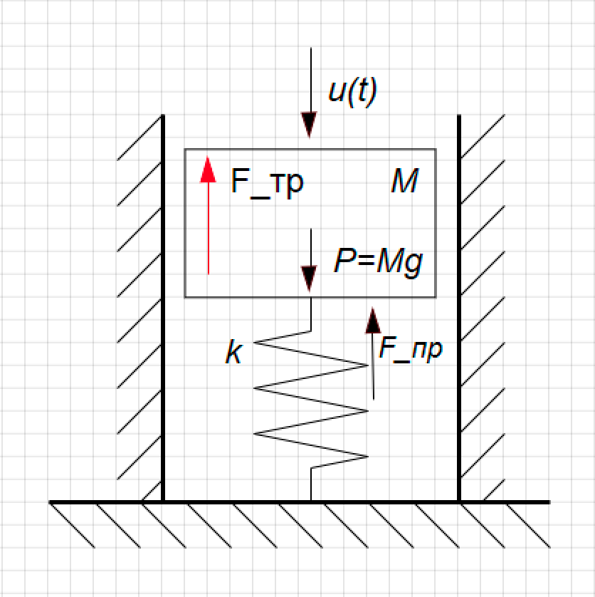
Figure 1. The design of the shock absorber.
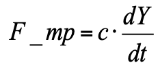
We derive the transfer function for this link.
Those Jedi who are already familiar with the magic of transfer functions can skip this part and go straight to expose the magic, and for the young Padawans we will reveal the whole technology for obtaining dynamic equations.
According to Newton's 2nd law, the acceleration of the body is proportional to the sum of the forces acting on the body:
 , (one)
where m is the body weight; F j - forces acting on the body (damper piston).
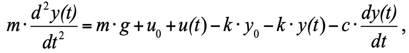
Substituting in equation (1) all the forces according to Fig. 1, we have:
 (2)
(2)
Where:
Y (t) is the position of the piston;
P = m ∙ g - gravity;
F_pr = k ∙ Y (t) - spring resistance force;
 - viscous friction force (proportional to the piston speed).
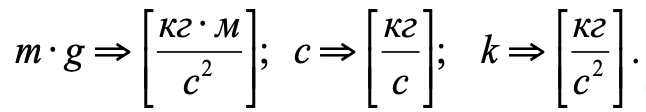
Dimensions of forces and coefficients included in equation (2):
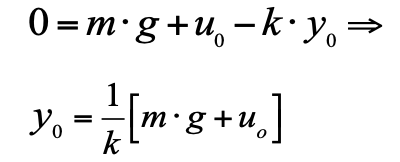
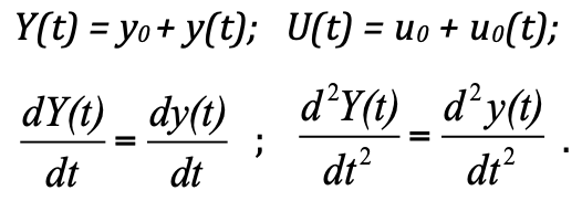
We believe that at zero time the piston is in equilibrium. Then the initial position of the piston is y 0 in equilibrium, where the velocity and acceleration are 0, can be calculated from equation 2.
This equation allows you to calculate in what position the piston will be at different loads. This static characteristic: applied force - received displacement. Its appearance for our system is extremely simple (see Fig. 2):
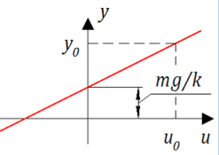
Figure 2. Static characteristic of the damper.
It would seem that here it is happiness - a simple line, when it applied force, it received displacement. But it was not there! We are not interested in the final position of the piston, but in the process of transition from one state to another.
To analyze the transition process, the theory of automatic control of TAU has been created. According to a typical "technology for creating models" according to this theory, it is proposed to consider the system not in absolute values, but in deviations from the equilibrium state. Such a statement simplifies the solution and construction. And in fact, if we replace the absolute values with deviations, we get:
F_pr = k ∙ (y 0 + y (t)) = k ∙ y 0 + k ∙ y (t) is the resistance force of the spring;
 - friction force.
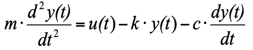
 but since we accepted that at the initial moment we have an equilibrium state, and the sum of the three forces in the equilibrium state is zero, we can remove them from the equation, and as a result we get:
 (four)
In order to translate the equation to the form according to the canon of TAU, it is necessary to divide the entire equation by k so that the coefficient y, the value of the output variable is equal to 1, and transfer the factors with output values of y (t) to the right side and the input values to the left side influences u (t) :
 (5)
(5)
This equation can already be written in operator form:
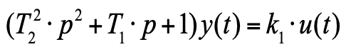 (6)
(6)
Where:

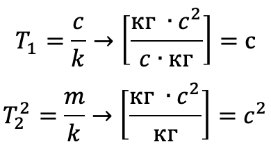
p = d / dt is the differentiation operator. Note that the dimensions of the coefficients have the dimension and meaning of time constants:
A transfer function for such an equation [6] has the form:

Now, before your very eyes, we got the transfer function in the form of a block from the equations of physics, and, moreover, the resulting block is a standard oscillatory link from TAU.
For me personally, the magic here is the magical appearance of static characteristics, parts of the system, mass of the piston, spring elasticity, friction on the walls) of the object magically appeared a temporary characteristic of transients in the system
As Maxim Andreev taught me, when creating dynamic models “The End is the Head for Everything!” ( See here the second principle of modeling - “start from the end” ):
And at the end of the function, we have a movement.
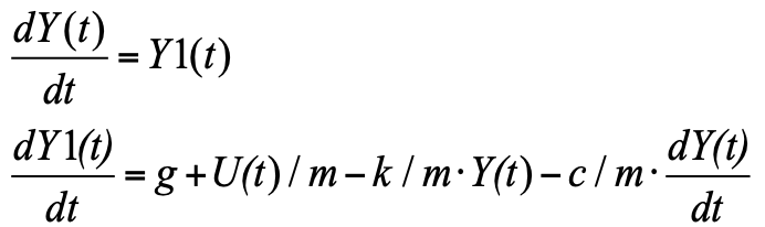
Therefore, Imagine Equation 2 in the form of Cauchy, to move.
The Cauchy form is when on the left are derivatives of the functions of interest to us, on the right are expressions for their calculation. Since the derivative in the equation is of the second degree, introducing a new variable Y1 - the rate of change of position (displacement velocity), we obtain a system of two equations in the form of Cauchy:
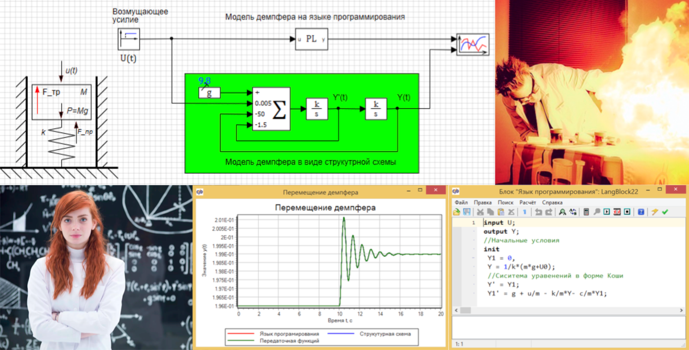
This equation can simply be written in the block "Programming language" and get a model (see Fig. 3):

Figure 3. A damper model in a programming language.
As an input, we use the value of force U, the output from the block is displacement Y, the initial position is given by formula 3. All variables are set as global signals for the project:
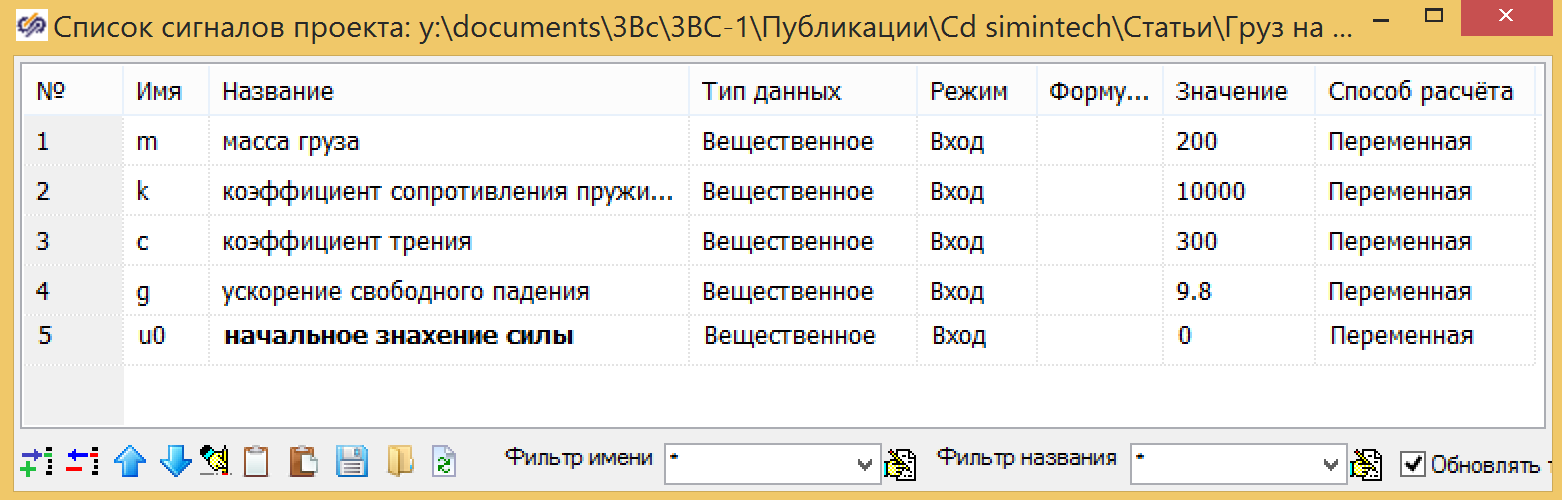
Figure 4. Global project variables.
The damper model can also be created in the form of a structure, in Figure 5, which shows a parallel damper model created from standard blocks, in which the initial condition is in the integrator at the output (see Fig. 6), and the coefficients are entered in the adder (see Fig. . 7)
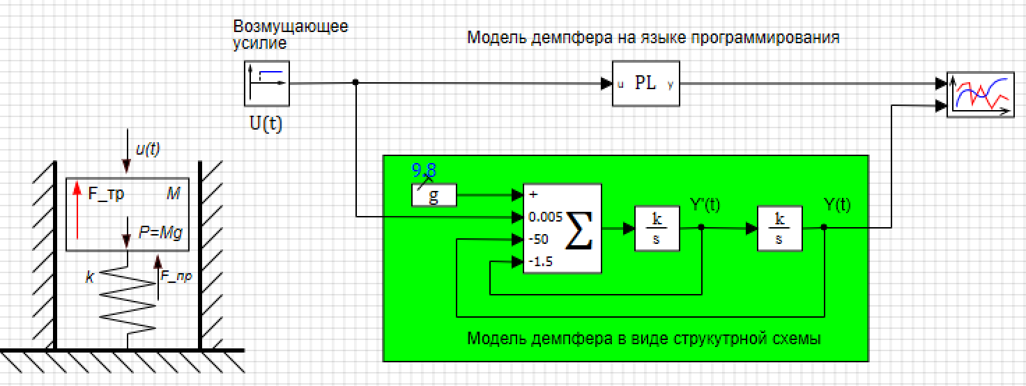
Figure 5. Damper in a programming language and in the form of a structural diagram.
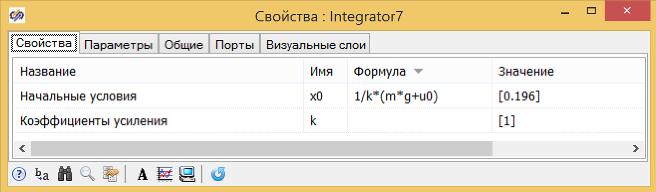
Figure 6. Integrator property with initial conditions.
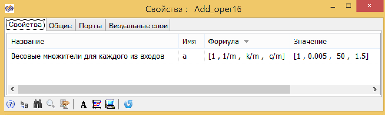
Figure 7. Properties of the adder with coefficients.
We set the perturbing action for 10 seconds, changing the acting force from 0 to 30, in a jump, and make sure that the two models show the same result (see Fig. 8).

Figure 8. Moving the damper.
Let's check the model in the form of a transfer function in a general form and in the form of an oscillating link, which this system is. To do this, we assemble the circuit, as shown in Figure 9.

Figure 9. Two damper models in the form of transfer functions.
It must be taken into account that we compiled the diagram in deviations, therefore, to obtain the absolute value, it is necessary to add a constant - the initial position of the piston.
For the transfer function (formula 7) we use the same global constants and expressions obtained previously for k 1 , T 1 , T 2 (see Fig. 10).
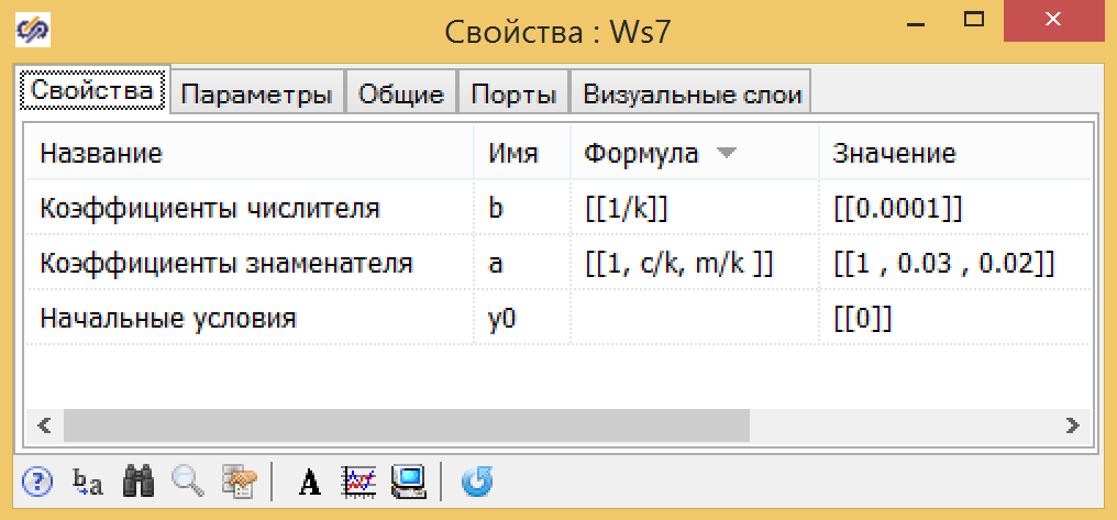
Figure 10. Parameters of the transfer function of the general form.
For the parameters of the vibrational link, the formulas are a little more complicated, but all can also be expressed in terms of global parameters: piston mass - m, spring drag coefficient - k, friction coefficient - s (see Fig. 11).
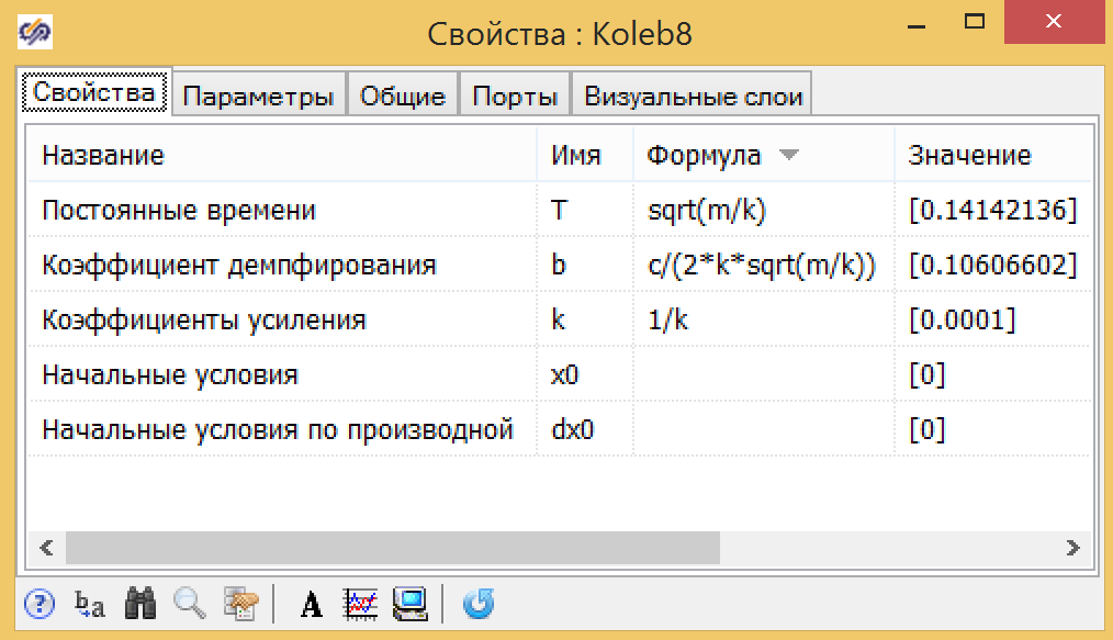
Figure 11. Parameters of the vibrational link.
Transition graphs show (see Figure 12) that TAU magic really works. The transfer function gives exactly the same results as a model based on equations of physics.
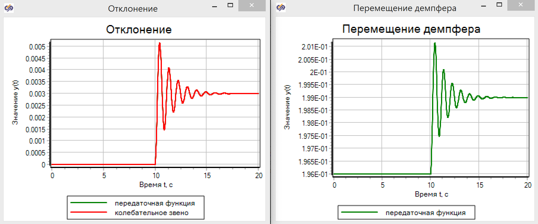
Figure 12. Moving the damper in TAU models.
Imagine that we do not have a model, and we use the identification unit according to the data obtained from the experiment. There is a whole technology of data analysis and transfer functions, but as part of the article and as an example, we will connect the transfer function building block to the model in the form of a programming language, as shown in Figure 13. We believe that we have a “black box” model, and we don’t know what is inside.

Figure 13. Connection scheme of the pseudo-identifier.
As a result of the analysis of our block in a programming language, we obtained a transfer function, which practically does not differ from the initial one, derived from the equations (see Fig. 14.). Compare with figure 10. Here it is a magic button!
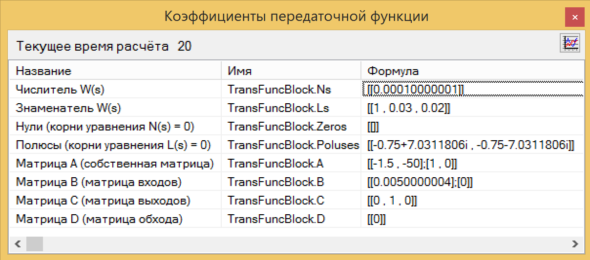
Figure 14. Identification results of the transfer function.
The numerator and denominator values can be directly copied from the identification block, pasted into the transfer function block and make sure that the graphs match. TAU magic works.
So why can't you always use System Identification for a model-oriented design process when everything is so magical?
To understand the lack of models obtained by identifying the System Identification black box, try to answer a simple question: what will be the deviation of the damper when the piston mass is increased by 30%?
And then it turns out that not all yogurts are equally useful.
In the event that you have honest equations, you simply change the mass of the load in the global variables of the project and get a new transition process, and a new transfer function.
In the case when, instead of honest equations of physics, you have a ready-made transfer function constructed from the results of the experiment, you need to run again and do the experiment to understand how the change in mass will affect the behavior of the model. As they say, a bad head does not give rest to legs.

The file with the damper model for experiments can be taken here ...
We presented the FAU2 missile model as a single transfer function, you can see it here ... And, it seems, everything worked. Why do we need to first study mathematical analysis and differential calculus when there is a magic button that gets the model from the tests?
Indeed, this approach can be applied, but this requires two conditions:
- The object should already be (not suitable for designed objects).
- Measurement data must be complete and reliable.
In any other cases - “they wanted the best, it turned out as always” (c).
For example, in this article about simulation of an electric drive, it is shown that “for a certain threshold value of the accuracy of measuring instruments, the drive model becomes unidentifiable, which leads to a loss of controllability and the inability to diagnose”
In the same article, we will analyze the magic and magic of creating models in the form of transfer functions from TAU, and then we will carry out a session of exposing this magic.
So first the magic
Let's take a look at a simple example. We have a model of mechanical damper. This is a piston on a spring, it moves inside the cylinder, it can move up and down. Its position is the function Y (t) that interests us, the disturbing force (U (t)) acts on it from above, and the force of viscous friction acts on the piston walls. (See Fig. 1)
Figure 1. The design of the shock absorber.
We derive the transfer function for this link.
Those Jedi who are already familiar with the magic of transfer functions can skip this part and go straight to expose the magic, and for the young Padawans we will reveal the whole technology for obtaining dynamic equations.
According to Newton's 2nd law, the acceleration of the body is proportional to the sum of the forces acting on the body:
, (one)
where m is the body weight; F j - forces acting on the body (damper piston).
Substituting in equation (1) all the forces according to Fig. 1, we have:
(2)
Where:
Y (t) is the position of the piston;
P = m ∙ g - gravity;
F_pr = k ∙ Y (t) - spring resistance force;
- viscous friction force (proportional to the piston speed).
Dimensions of forces and coefficients included in equation (2):
We believe that at zero time the piston is in equilibrium. Then the initial position of the piston is y 0 in equilibrium, where the velocity and acceleration are 0, can be calculated from equation 2.
This equation allows you to calculate in what position the piston will be at different loads. This static characteristic: applied force - received displacement. Its appearance for our system is extremely simple (see Fig. 2):
Figure 2. Static characteristic of the damper.
It would seem that here it is happiness - a simple line, when it applied force, it received displacement. But it was not there! We are not interested in the final position of the piston, but in the process of transition from one state to another.
To analyze the transition process, the theory of automatic control of TAU has been created. According to a typical "technology for creating models" according to this theory, it is proposed to consider the system not in absolute values, but in deviations from the equilibrium state. Such a statement simplifies the solution and construction. And in fact, if we replace the absolute values with deviations, we get:
F_pr = k ∙ (y 0 + y (t)) = k ∙ y 0 + k ∙ y (t) is the resistance force of the spring;
- friction force.
but since we accepted that at the initial moment we have an equilibrium state, and the sum of the three forces in the equilibrium state is zero, we can remove them from the equation, and as a result we get:
(four)
In order to translate the equation to the form according to the canon of TAU, it is necessary to divide the entire equation by k so that the coefficient y, the value of the output variable is equal to 1, and transfer the factors with output values of y (t) to the right side and the input values to the left side influences u (t) :
(5)
This equation can already be written in operator form:
(6)
Where:
p = d / dt is the differentiation operator. Note that the dimensions of the coefficients have the dimension and meaning of time constants:
A transfer function for such an equation [6] has the form:
Now, before your very eyes, we got the transfer function in the form of a block from the equations of physics, and, moreover, the resulting block is a standard oscillatory link from TAU.
For me personally, the magic here is the magical appearance of static characteristics, parts of the system, mass of the piston, spring elasticity, friction on the walls) of the object magically appeared a temporary characteristic of transients in the system
Check the formulas with the model
As Maxim Andreev taught me, when creating dynamic models “The End is the Head for Everything!” ( See here the second principle of modeling - “start from the end” ):
And at the end of the function, we have a movement.
Therefore, Imagine Equation 2 in the form of Cauchy, to move.
The Cauchy form is when on the left are derivatives of the functions of interest to us, on the right are expressions for their calculation. Since the derivative in the equation is of the second degree, introducing a new variable Y1 - the rate of change of position (displacement velocity), we obtain a system of two equations in the form of Cauchy:
This equation can simply be written in the block "Programming language" and get a model (see Fig. 3):
Figure 3. A damper model in a programming language.
As an input, we use the value of force U, the output from the block is displacement Y, the initial position is given by formula 3. All variables are set as global signals for the project:
Figure 4. Global project variables.
The damper model can also be created in the form of a structure, in Figure 5, which shows a parallel damper model created from standard blocks, in which the initial condition is in the integrator at the output (see Fig. 6), and the coefficients are entered in the adder (see Fig. . 7)
Figure 5. Damper in a programming language and in the form of a structural diagram.
Figure 6. Integrator property with initial conditions.
Figure 7. Properties of the adder with coefficients.
We set the perturbing action for 10 seconds, changing the acting force from 0 to 30, in a jump, and make sure that the two models show the same result (see Fig. 8).
Figure 8. Moving the damper.
Let's check the model in the form of a transfer function in a general form and in the form of an oscillating link, which this system is. To do this, we assemble the circuit, as shown in Figure 9.
Figure 9. Two damper models in the form of transfer functions.
It must be taken into account that we compiled the diagram in deviations, therefore, to obtain the absolute value, it is necessary to add a constant - the initial position of the piston.
For the transfer function (formula 7) we use the same global constants and expressions obtained previously for k 1 , T 1 , T 2 (see Fig. 10).
Figure 10. Parameters of the transfer function of the general form.
For the parameters of the vibrational link, the formulas are a little more complicated, but all can also be expressed in terms of global parameters: piston mass - m, spring drag coefficient - k, friction coefficient - s (see Fig. 11).
Figure 11. Parameters of the vibrational link.
Transition graphs show (see Figure 12) that TAU magic really works. The transfer function gives exactly the same results as a model based on equations of physics.
Figure 12. Moving the damper in TAU models.
Imagine that we do not have a model, and we use the identification unit according to the data obtained from the experiment. There is a whole technology of data analysis and transfer functions, but as part of the article and as an example, we will connect the transfer function building block to the model in the form of a programming language, as shown in Figure 13. We believe that we have a “black box” model, and we don’t know what is inside.
Figure 13. Connection scheme of the pseudo-identifier.
As a result of the analysis of our block in a programming language, we obtained a transfer function, which practically does not differ from the initial one, derived from the equations (see Fig. 14.). Compare with figure 10. Here it is a magic button!
Figure 14. Identification results of the transfer function.
The numerator and denominator values can be directly copied from the identification block, pasted into the transfer function block and make sure that the graphs match. TAU magic works.
Session of exposing magic
So why can't you always use System Identification for a model-oriented design process when everything is so magical?
To understand the lack of models obtained by identifying the System Identification black box, try to answer a simple question: what will be the deviation of the damper when the piston mass is increased by 30%?
And then it turns out that not all yogurts are equally useful.
In the event that you have honest equations, you simply change the mass of the load in the global variables of the project and get a new transition process, and a new transfer function.
In the case when, instead of honest equations of physics, you have a ready-made transfer function constructed from the results of the experiment, you need to run again and do the experiment to understand how the change in mass will affect the behavior of the model. As they say, a bad head does not give rest to legs.
Findings:
- Sitting down and thinking about the equations of physics is always more useful and cheaper than experimenting.
- A model derived from the physical equations of processes is much tastier and more useful than transfer functions.
- The experiment should clarify unknown coefficients or difficult to measure parameters.
- Learn physics and you will be happy!
The file with the damper model for experiments can be taken here ...
All Articles