The full course in Russian can be found at this link .

The original English course is available at this link .

Content

1. Interview with Sebastian Trun
2. Introduction
3. Transfer Learning Model
4. MobileNet
5. CoLab: Cats Vs Dogs with Training Transfer
6. Diving into convolutional neural networks
7. Practical part: determination of colors with the transfer of training
8. Summary

Interview with Sebastian Trun

- This is lesson 6 and it is completely dedicated to transfer learning. Learning transfer is the process of using an existing model with little refinement for new tasks. The transfer of training helps to reduce the training time of the model by giving some increase in efficiency when learning at the very beginning. Sebastian, what do you think about the transfer of training? Have you ever been able to use the teaching transfer methodology in your work and research?

- My dissertation was devoted just to the topic of transfer of training and was called " Explanation on the basis of transfer of training ." When we were working on a dissertation, the idea was that it is possible to teach to distinguish all other objects of this kind on one object (data set, entity) in various variations and formats. In the work, we used the developed algorithm, which distinguished the main characteristics (attributes) of the object and could compare them with another object. Libraries like Tensorflow already come with pre-trained models.

- Yes, at Tensorflow we have a complete set of pre-trained models that you can use to solve practical problems. We will talk about ready-made sets a little later.

- Yes Yes! If you think about it, then people are engaged in the transfer of training all the time throughout their lives.

- Can we say that thanks to the method of transferring training, our new students at some point will not have to know something about machine learning because it will be enough to connect an already prepared model and use it?

- Programming is writing line by line, we give commands to the computer. Our goal is to make sure that everyone on the planet is able and able to program by providing the computer with only examples of input data. Agree, if you want to teach a computer to distinguish cats from dogs, then finding 100k different images of cats and 100k different images of dogs is quite difficult, and thanks to the transfer of training you can solve this problem in several lines.

- Yes this is true! Thank you for the answers and let's finally move on to learning.

Introduction

- Hello and welcome back!

- Last time we trained the convolutional neural network to classify cats and dogs in the image. Our first neural network was retrained, so its result was not so high - about 70% accuracy. After that, we implemented data extension and dropout (arbitrary disconnection of neurons), which allowed us to increase the accuracy of predictions up to 80%.

- Despite the fact that 80% may seem like an excellent indicator, the 20% error is still too large. Is not it? What can we do to increase the accuracy of the classification? In this lesson, we will use the knowledge transfer technique (transfer of the knowledge model), which will allow us to use the model developed by experts and trained on huge data arrays. As we will see in practice, by transferring the knowledge model we can achieve 95% classification accuracy. Let's get started!

Learning Model Transfer

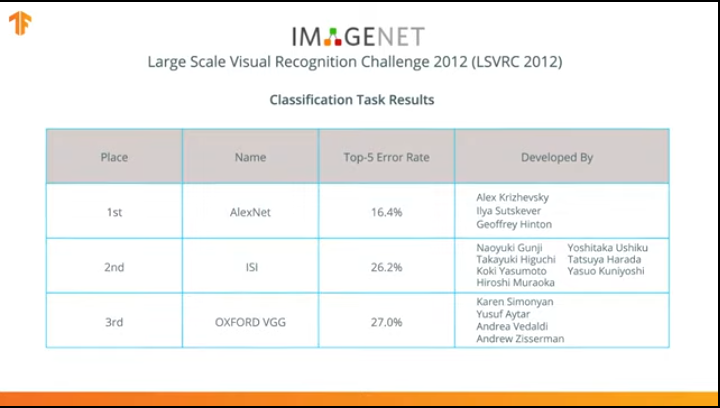
In 2012, the AlexNet neural network revolutionized the world of machine learning and popularized the use of convolutional neural networks for classification by winning the ImageNet Large Scale Visual recognition challenge.

After that, the struggle began to develop more accurate and efficient neural networks that could surpass AlexNet in the tasks of classifying images from the ImageNet dataset.

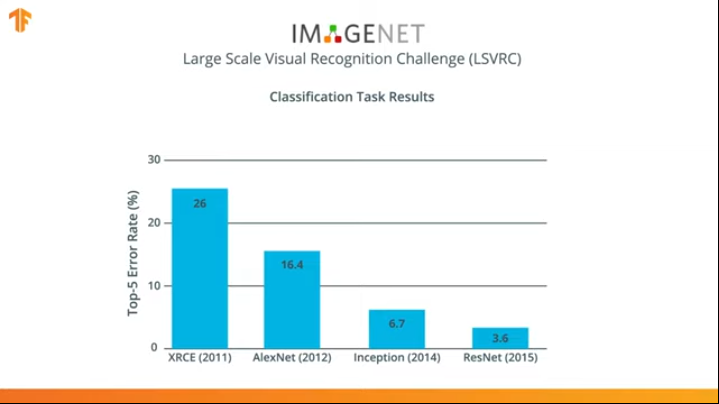
For several years, neural networks have been developed that cope with the classification task better than AlexNet - Inception and ResNet.

Agree that it would be great to be able to use these neural networks, already trained on huge datasets from ImageNet, and use them in your classifier for cats and dogs?

It turns out that we can do it! The technique is called transfer learning. The main idea of ​​the method of transferring the training model is based on the fact that having trained a neural network on a large data set, we can apply the obtained model to a data set that this model has not yet encountered. That is why the technique is called transfer learning - transferring the learning process from one data set to another.

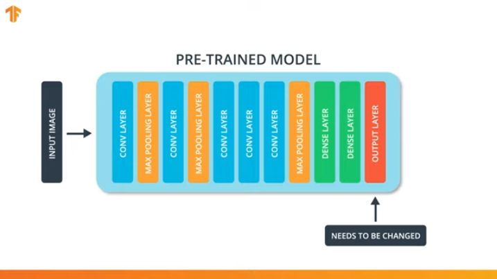
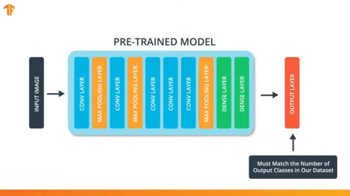
In order for us to apply the training model transfer methodology, we need to change the last layer of our convolutional neural network:

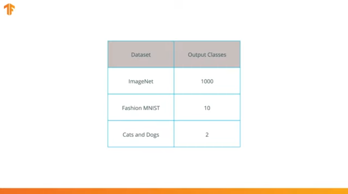
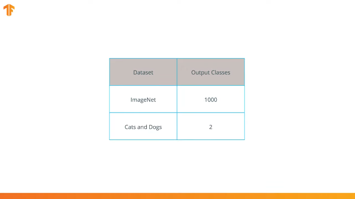
We perform this operation because each data set consists of a different number of output classes. For example, datasets in ImageNet contain 1000 different output classes. FashionMNIST contains 10 classes. Our classification dataset consists of only 2 classes - cats and dogs.

That is why it is necessary to change the last layer of our convolutional neural network so that it contains the number of outputs that would correspond to the number of classes in the new set.

We also need to make sure that we do not change the pre-trained model during the training process. The solution is to turn off the variables of the pre-trained model - we simply prohibit the algorithm from updating the values ​​during forward and backward propagation to change them.

This process is called the “freezing the model”.

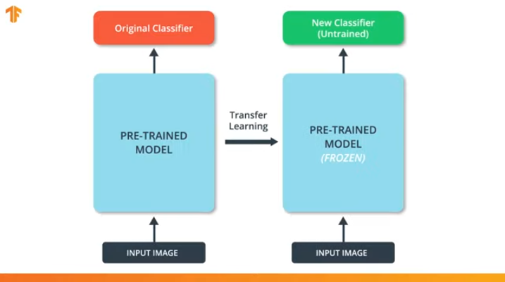
By “freezing” the parameters of the pre-trained model, we allow learning only the last layer of the classification network, the values ​​of the variables of the pre-trained model remain unchanged.

Another indisputable advantage of pre-trained models is that we reduce the training time by training only the last layer with a significantly smaller number of variables, and not the entire model.

If we do not “freeze” the variables of the pre-trained model, then in the process of training on the new data set the values ​​of the variables will change. This is because the values ​​of the variables on the last layer of the classification will be filled with random values. Due to random values ​​on the last layer, our model will make big mistakes in the classification, which, in turn, will entail strong changes in the initial weights in the pre-trained model, which is extremely undesirable for us.

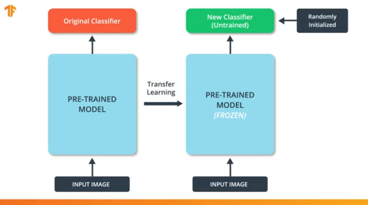
It is for this reason that we should always remember that when using existing models, the values ​​of variables should be “frozen" and the need to train a pre-trained model should be turned off.

Now that we know how the transfer of the training model works, we just have to choose a pre-trained neural network for use in our own classifier! This we will do in the next part.

MobileNet

As we mentioned earlier, extremely efficient neural networks were developed that showed high results on ImageNet datasets - AlexNet, Inception, Resonant. These neural networks are very deep networks and contain thousands and even millions of parameters. A large number of parameters allows the network to learn more complex patterns and thereby achieve increased classification accuracy. A large number of training parameters of the neural network affects the speed of learning, the amount of memory required to store the network and the complexity of the calculations.

In this lesson we will use the modern convolutional neural network MobileNet. MobileNet is an efficient convolutional neural network architecture that reduces the amount of memory used for computing while maintaining high accuracy of predictions. That is why MobileNet is ideal for use on mobile devices with a limited amount of memory and computing resources.

MobileNet was developed by Google and trained on the ImageNet dataset.

Since MobileNet was trained in 1,000 classes from the ImageNet dataset, MobileNet has 1,000 output classes, instead of the two we need - a cat and a dog.

To complete the transfer of training, we preload the feature vector without a classification layer:

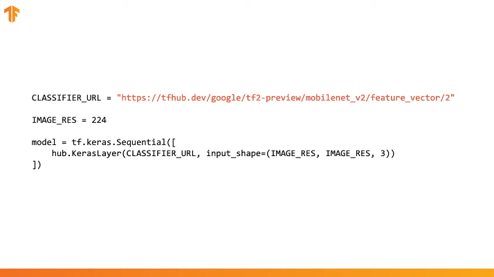
In Tensorflow, a loaded feature vector can be used as a regular Keras layer with input data of a certain size.

Since MobileNet was trained on the ImageNet dataset, we will need to bring the size of the input data to those that were used in the training process. In our case, MobileNet was trained on 224x224px fixed-size RGB images.

TensorFlow contains a pre-trained repository called TensorFlow Hub.

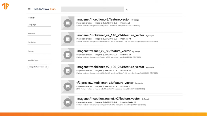
TensorFlow Hub contains some pre-trained models in which the last classification layer was excluded from the neural network architecture for subsequent reuse.

You can use the TensorFlow Hub in the code in several lines:

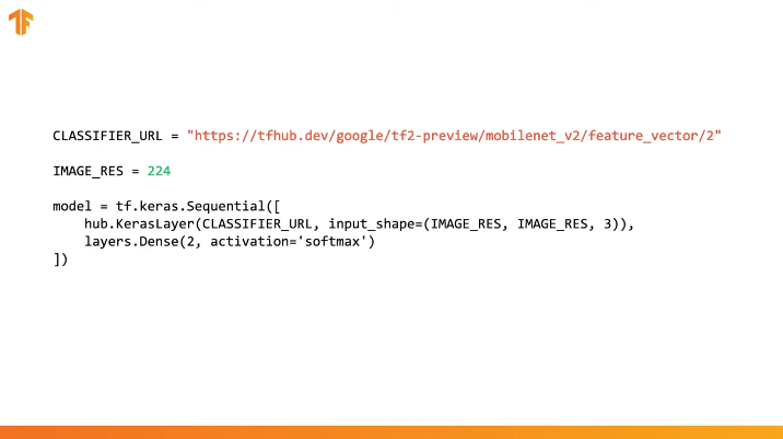
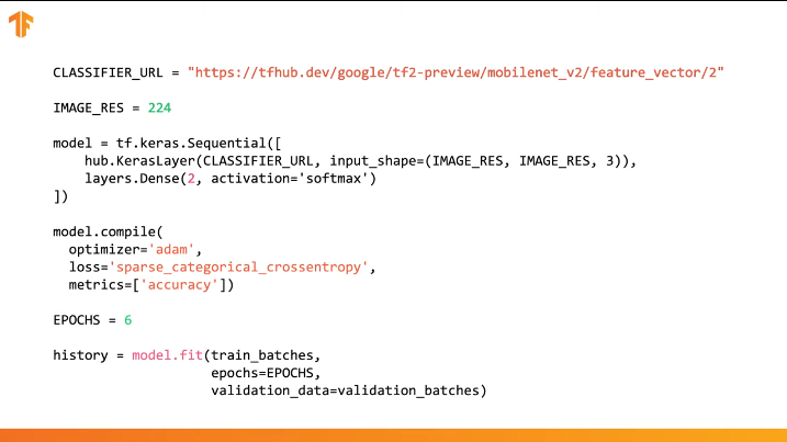
It is enough to specify the URL of the feature vector of the desired training model and then embed the model in our classifier with the last layer with the desired number of output classes. It is the last layer that will be subjected to training and changing parameter values. Compilation and training of our new model is carried out in the same way as we did before:

Let's see how this will actually work and write the appropriate code.

CoLab: Cats Vs Dogs with Training Transfer

Link to CoLab in Russian and CoLab in English .

TensorFlow Hub is a repository with pre-trained models that we can use.

Learning transfer is a process in which we take a pre-trained model and expand it to perform a specific task. At the same time, we leave the part of the pre-trained model that we integrate into the neural network untouched, but only train the last output layers to obtain the desired result.

In this practical part, we will test both options.

This link allows you to explore the entire list of available models.

In this part of Colab

1. We will use the TensorFlow Hub model for predictions;
2. We will use the TensorFlow Hub-model for the data set of cats and dogs;
3. Let's transfer the training using the model from the TensorFlow Hub.

Before proceeding with the implementation of the current practical part, we recommend resetting the Runtime -> Reset all runtimes...

Library Imports

In this practical part, we will use a number of TensorFlow library features that are not yet in the official release. That is why we will first install the TensorFlow and TensorFlow Hub version for developers.

Installing the dev version of TensorFlow automatically activates the latest installed version. After we finish dealing with this practical part, we recommend restoring the TensorFlow settings and returning to the stable version via the menu item Runtime -> Reset all runtimes...



Executing this command will reset all environment settings to the initial ones.

 !pip install tf-nightly-gpu !pip install "tensorflow_hub==0.4.0" !pip install -U tensorflow_datasets
      
      

        
        
        
      

    
        
        
        
      
      

        
        
        
      

    
     

Output:

 Requirement already satisfied: absl-py>=0.7.0 in /usr/local/lib/python3.6/dist-packages (from tf-nightly-gpu) (0.8.0) Requirement already satisfied: protobuf>=3.6.1 in /usr/local/lib/python3.6/dist-packages (from tf-nightly-gpu) (3.7.1) Requirement already satisfied: google-pasta>=0.1.6 in /usr/local/lib/python3.6/dist-packages (from tf-nightly-gpu) (0.1.7) Collecting tf-estimator-nightly (from tf-nightly-gpu) Downloading https://files.pythonhosted.org/packages/ea/72/f092fc631ef2602fd0c296dcc4ef6ef638a6a773cb9fdc6757fecbfffd33/tf_estimator_nightly-1.14.0.dev2019092201-py2.py3-none-any.whl (450kB) |████████████████████████████████| 450kB 45.9MB/s Requirement already satisfied: numpy<2.0,>=1.16.0 in /usr/local/lib/python3.6/dist-packages (from tf-nightly-gpu) (1.16.5) Requirement already satisfied: wrapt>=1.11.1 in /usr/local/lib/python3.6/dist-packages (from tf-nightly-gpu) (1.11.2) Requirement already satisfied: astor>=0.6.0 in /usr/local/lib/python3.6/dist-packages (from tf-nightly-gpu) (0.8.0) Requirement already satisfied: opt-einsum>=2.3.2 in /usr/local/lib/python3.6/dist-packages (from tf-nightly-gpu) (3.0.1) Requirement already satisfied: wheel>=0.26 in /usr/local/lib/python3.6/dist-packages (from tf-nightly-gpu) (0.33.6) Requirement already satisfied: h5py in /usr/local/lib/python3.6/dist-packages (from keras-applications>=1.0.8->tf-nightly-gpu) (2.8.0) Requirement already satisfied: markdown>=2.6.8 in /usr/local/lib/python3.6/dist-packages (from tb-nightly<1.16.0a0,>=1.15.0a0->tf-nightly-gpu) (3.1.1) Requirement already satisfied: setuptools>=41.0.0 in /usr/local/lib/python3.6/dist-packages (from tb-nightly<1.16.0a0,>=1.15.0a0->tf-nightly-gpu) (41.2.0) Requirement already satisfied: werkzeug>=0.11.15 in /usr/local/lib/python3.6/dist-packages (from tb-nightly<1.16.0a0,>=1.15.0a0->tf-nightly-gpu) (0.15.6) Installing collected packages: tb-nightly, tf-estimator-nightly, tf-nightly-gpu Successfully installed tb-nightly-1.15.0a20190911 tf-estimator-nightly-1.14.0.dev2019092201 tf-nightly-gpu-1.15.0.dev20190821 Collecting tensorflow_hub==0.4.0 Downloading https://files.pythonhosted.org/packages/10/5c/6f3698513cf1cd730a5ea66aec665d213adf9de59b34f362f270e0bd126f/tensorflow_hub-0.4.0-py2.py3-none-any.whl (75kB) |████████████████████████████████| 81kB 5.0MB/s Requirement already satisfied: protobuf>=3.4.0 in /usr/local/lib/python3.6/dist-packages (from tensorflow_hub==0.4.0) (3.7.1) Requirement already satisfied: numpy>=1.12.0 in /usr/local/lib/python3.6/dist-packages (from tensorflow_hub==0.4.0) (1.16.5) Requirement already satisfied: six>=1.10.0 in /usr/local/lib/python3.6/dist-packages (from tensorflow_hub==0.4.0) (1.12.0) Requirement already satisfied: setuptools in /usr/local/lib/python3.6/dist-packages (from protobuf>=3.4.0->tensorflow_hub==0.4.0) (41.2.0) Installing collected packages: tensorflow-hub Found existing installation: tensorflow-hub 0.6.0 Uninstalling tensorflow-hub-0.6.0: Successfully uninstalled tensorflow-hub-0.6.0 Successfully installed tensorflow-hub-0.4.0 Collecting tensorflow_datasets Downloading https://files.pythonhosted.org/packages/6c/34/ff424223ed4331006aaa929efc8360b6459d427063dc59fc7b75d7e4bab3/tensorflow_datasets-1.2.0-py3-none-any.whl (2.3MB) |████████████████████████████████| 2.3MB 4.9MB/s Requirement already satisfied, skipping upgrade: future in /usr/local/lib/python3.6/dist-packages (from tensorflow_datasets) (0.16.0) Requirement already satisfied, skipping upgrade: wrapt in /usr/local/lib/python3.6/dist-packages (from tensorflow_datasets) (1.11.2) Requirement already satisfied, skipping upgrade: dill in /usr/local/lib/python3.6/dist-packages (from tensorflow_datasets) (0.3.0) Requirement already satisfied, skipping upgrade: numpy in /usr/local/lib/python3.6/dist-packages (from tensorflow_datasets) (1.16.5) Requirement already satisfied, skipping upgrade: requests>=2.19.0 in /usr/local/lib/python3.6/dist-packages (from tensorflow_datasets) (2.21.0) Requirement already satisfied, skipping upgrade: tqdm in /usr/local/lib/python3.6/dist-packages (from tensorflow_datasets) (4.28.1) Requirement already satisfied, skipping upgrade: protobuf>=3.6.1 in /usr/local/lib/python3.6/dist-packages (from tensorflow_datasets) (3.7.1) Requirement already satisfied, skipping upgrade: psutil in /usr/local/lib/python3.6/dist-packages (from tensorflow_datasets) (5.4.8) Requirement already satisfied, skipping upgrade: promise in /usr/local/lib/python3.6/dist-packages (from tensorflow_datasets) (2.2.1) Requirement already satisfied, skipping upgrade: absl-py in /usr/local/lib/python3.6/dist-packages (from tensorflow_datasets) (0.8.0) Requirement already satisfied, skipping upgrade: tensorflow-metadata in /usr/local/lib/python3.6/dist-packages (from tensorflow_datasets) (0.14.0) Requirement already satisfied, skipping upgrade: six in /usr/local/lib/python3.6/dist-packages (from tensorflow_datasets) (1.12.0) Requirement already satisfied, skipping upgrade: termcolor in /usr/local/lib/python3.6/dist-packages (from tensorflow_datasets) (1.1.0) Requirement already satisfied, skipping upgrade: attrs in /usr/local/lib/python3.6/dist-packages (from tensorflow_datasets) (19.1.0) Requirement already satisfied, skipping upgrade: idna<2.9,>=2.5 in /usr/local/lib/python3.6/dist-packages (from requests>=2.19.0->tensorflow_datasets) (2.8) Requirement already satisfied, skipping upgrade: certifi>=2017.4.17 in /usr/local/lib/python3.6/dist-packages (from requests>=2.19.0->tensorflow_datasets) (2019.6.16) Requirement already satisfied, skipping upgrade: chardet<3.1.0,>=3.0.2 in /usr/local/lib/python3.6/dist-packages (from requests>=2.19.0->tensorflow_datasets) (3.0.4) Requirement already satisfied, skipping upgrade: urllib3<1.25,>=1.21.1 in /usr/local/lib/python3.6/dist-packages (from requests>=2.19.0->tensorflow_datasets) (1.24.3) Requirement already satisfied, skipping upgrade: setuptools in /usr/local/lib/python3.6/dist-packages (from protobuf>=3.6.1->tensorflow_datasets) (41.2.0) Requirement already satisfied, skipping upgrade: googleapis-common-protos in /usr/local/lib/python3.6/dist-packages (from tensorflow-metadata->tensorflow_datasets) (1.6.0) Installing collected packages: tensorflow-datasets Successfully installed tensorflow-datasets-1.2.0
      
      

        
        
        
      

    
        
        
        
      
      

        
        
        
      

    
     

We have already seen and used some imports before. From the new - import tensorflow_hub



, which we installed and which we will use in this practical part.

 from __future__ import absolute_import, division, print_function, unicode_literals import matplotlib.pylab as plt import tensorflow as tf tf.enable_eager_execution() import tensorflow_hub as hub import tensorflow_datasets as tfds from tensorflow.keras import layers
      
      

        
        
        
      

    
        
        
        
      
      

        
        
        
      

    
     

Output:

 WARNING:tensorflow: TensorFlow's `tf-nightly` package will soon be updated to TensorFlow 2.0. Please upgrade your code to TensorFlow 2.0: * https://www.tensorflow.org/beta/guide/migration_guide Or install the latest stable TensorFlow 1.X release: * `pip install -U "tensorflow==1.*"` Otherwise your code may be broken by the change.
      
      

        
        
        
      

    
        
        
        
      
      

        
        
        
      

    
     

 import logging logger = tf.get_logger() logger.setLevel(logging.ERROR)
      
      

        
        
        
      

    
        
        
        
      
      

        
        
        
      

    
     

Part 1: using the TensorFlow Hub MobileNet for predictions

In this part of CoLab, we will take a pre-trained model, upload it to Keras and test it.

The model we are using is MobileNet v2 (instead of MobileNet, any other tf2 compatible image classifier model with tfhub.dev can be used).

Download classifier

Download the MobileNet model and create a Keras model from it. MobileNet at the input expects to receive an image of 224x224 pixels in size with 3 color channels (RGB).

 CLASSIFIER_URL = "https://tfhub.dev/google/tf2-preview/mobilenet_v2/classification/2" IMAGE_RES = 224 model = tf.keras.Sequential([ hub.KerasLayer(CLASSIFIER_URL, input_shape=(IMAGE_RES, IMAGE_RES, 3)) ])
      
      

        
        
        
      

    
        
        
        
      
      

        
        
        
      

    
     

Run the classifier on a single image

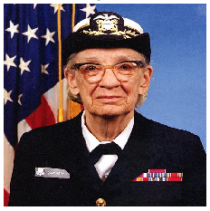
MobileNet has been trained on the ImageNet dataset. ImageNet contains 1000 output classes and one of these classes is military uniform. Let's find the image on which the military uniform will be located and which will not be part of the ImageNet training kit to verify the classification accuracy.

 import numpy as np import PIL.Image as Image grace_hopper = tf.keras.utils.get_file('image.jpg', 'https://storage.googleapis.com/download.tensorflow.org/example_images/grace_hopper.jpg') grace_hopper = Image.open(grace_hopper).resize((IMAGE_RES, IMAGE_RES)) grace_hopper
      
      

        
        
        
      

    
        
        
        
      
      

        
        
        
      

    
     

Output:

 Downloading data from https://storage.googleapis.com/download.tensorflow.org/example_images/grace_hopper.jpg 65536/61306 [================================] - 0s 0us/step
      
      

        
        
        
      

    
        
        
        
      
      

        
        
        
      

    
     

 grace_hopper = np.array(grace_hopper)/255.0 grace_hopper.shape
      
      

        
        
        
      

    
        
        
        
      
      

        
        
        
      

    
     

Output:

 (224, 224, 3)
      
      

        
        
        
      

    
        
        
        
      
      

        
        
        
      

    
     

Keep in mind that models always receive a set (block) of images for processing at the input. In the code below, we add a new dimension - the block size.

 result = model.predict(grace_hopper[np.newaxis, ...]) result.shape
      
      

        
        
        
      

    
        
        
        
      
      

        
        
        
      

    
     

Output:

 (1, 1001)
      
      

        
        
        
      

    
        
        
        
      
      

        
        
        
      

    
     

The result of the prediction was a vector with a size of 1,001 elements, where each value represents the probability that the object in the image belongs to a certain class.

The position of the maximum probability value can be found using the argmax



function. However, there is a question that we still have not answered - how can we determine which class an element belongs to with maximum probability?

 predicted_class = np.argmax(result[0], axis=-1) predicted_class
      
      

        
        
        
      

    
        
        
        
      
      

        
        
        
      

    
     

Output:

 653
      
      

        
        
        
      

    
        
        
        
      
      

        
        
        
      

    
     

Deciphering Predictions

In order for us to determine the class to which the predictions relate, we upload the list of ImageNet tags and by the index with maximum fidelity we determine the class to which the prediction relates.

 labels_path = tf.keras.utils.get_file('ImageNetLabels.txt','https://storage.googleapis.com/download.tensorflow.org/data/ImageNetLabels.txt') imagenet_labels = np.array(open(labels_path).read().splitlines()) plt.imshow(grace_hopper) plt.axis('off') predicted_class_name = imagenet_labels[predicted_class] _ = plt.title("Prediction: " + predicted_class_name.title())
      
      

        
        
        
      

    
        
        
        
      
      

        
        
        
      

    
     

Output:

 Downloading data from https://storage.googleapis.com/download.tensorflow.org/data/ImageNetLabels.txt 16384/10484 [==============================================] - 0s 0us/step
      
      

        
        
        
      

    
        
        
        
      
      

        
        
        
      

    
     

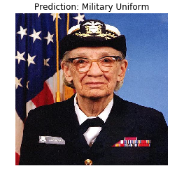
Bingo! Our model correctly identified the military uniform.

Part 2: use the TensorFlow Hub model for a cat and dog dataset

Now we will use the full version of the MobileNet model and see how it will cope with the data set of cats and dogs.

Data set

We can use TensorFlow Datasets to download a cat and dog dataset.

 splits = tfds.Split.ALL.subsplit(weighted=(80, 20)) splits, info = tfds.load('cats_vs_dogs', with_info=True, as_supervised=True, split = splits) (train_examples, validation_examples) = splits num_examples = info.splits['train'].num_examples num_classes = info.features['label'].num_classes
      
      

        
        
        
      

    
        
        
        
      
      

        
        
        
      

    
     

Output:

 Downloading and preparing dataset cats_vs_dogs (786.68 MiB) to /root/tensorflow_datasets/cats_vs_dogs/2.0.1... /usr/local/lib/python3.6/dist-packages/urllib3/connectionpool.py:847: InsecureRequestWarning: Unverified HTTPS request is being made. Adding certificate verification is strongly advised. See: https://urllib3.readthedocs.io/en/latest/advanced-usage.html#ssl-warnings InsecureRequestWarning) WARNING:absl:1738 images were corrupted and were skipped Dataset cats_vs_dogs downloaded and prepared to /root/tensorflow_datasets/cats_vs_dogs/2.0.1. Subsequent calls will reuse this data.
      
      

        
        
        
      

    
        
        
        
      
      

        
        
        
      

    
     

Not all images in a cat and dog dataset are the same size.

 for i, example_image in enumerate(train_examples.take(3)): print("Image {} shape: {}".format(i+1, example_image[0].shape))
      
      

        
        
        
      

    
        
        
        
      
      

        
        
        
      

    
     

Output:

 Image 1 shape: (500, 343, 3) Image 2 shape: (375, 500, 3) Image 3 shape: (375, 500, 3)
      
      

        
        
        
      

    
        
        
        
      
      

        
        
        
      

    
     

Therefore, images from the obtained data set require reduction to a single size, which the MobileNet model expects at the input - 224 x 224.

The .repeat()



function and steps_per_epoch



are not required here, but they allow saving about 15 seconds for each training iteration, because the temporary buffer has to be initialized only once at the very beginning of the learning process.

 def format_image(image, label): image = tf.image.resize(image, (IMAGE_RES, IMAGE_RES)) / 255.0 return image, label BATCH_SIZE = 32 train_batches = train_examples.shuffle(num_examples//4).map(format_image).batch(BATCH_SIZE).prefetch(1) validation_batches = validation_examples.map(format_image).batch(BATCH_SIZE).prefetch(1)
      
      

        
        
        
      

    
        
        
        
      
      

        
        
        
      

    
     

Run the classifier on image sets

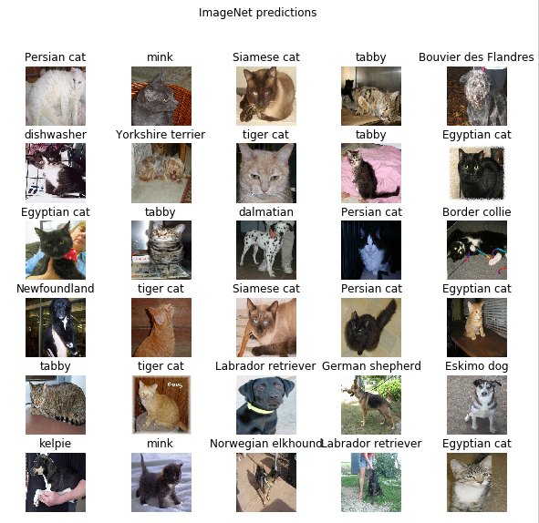
Let me remind you that at this stage, there is still a full version of the pre-trained MobileNet network, which contains 1,000 possible output classes. ImageNet contains a large number of images of dogs and cats, so let's try to input one of the test images from our data set and see what prediction the model will give us.

 image_batch, label_batch = next(iter(train_batches.take(1))) image_batch = image_batch.numpy() label_batch = label_batch.numpy() result_batch = model.predict(image_batch) predicted_class_names = imagenet_labels[np.argmax(result_batch, axis=-1)] predicted_class_names
      
      

        
        
        
      

    
        
        
        
      
      

        
        
        
      

    
     

Output:

 array(['Persian cat', 'mink', 'Siamese cat', 'tabby', 'Bouvier des Flandres', 'dishwasher', 'Yorkshire terrier', 'tiger cat', 'tabby', 'Egyptian cat', 'Egyptian cat', 'tabby', 'dalmatian', 'Persian cat', 'Border collie', 'Newfoundland', 'tiger cat', 'Siamese cat', 'Persian cat', 'Egyptian cat', 'tabby', 'tiger cat', 'Labrador retriever', 'German shepherd', 'Eskimo dog', 'kelpie', 'mink', 'Norwegian elkhound', 'Labrador retriever', 'Egyptian cat', 'computer keyboard', 'boxer'], dtype='<U30')
      
      

        
        
        
      

    
        
        
        
      
      

        
        
        
      

    
     

Labels are similar to cat and dog breeds. Let's now display some images from our cats and dogs dataset and place a predicted label on each of them.

 plt.figure(figsize=(10, 9)) for n in range(30): plt.subplot(6, 5, n+1) plt.subplots_adjust(hspace=0.3) plt.imshow(image_batch[n]) plt.title(predicted_class_names[n]) plt.axis('off') _ = plt.suptitle("ImageNet predictions")
      
      

        
        
        
      

    
        
        
        
      
      

        
        
        
      

    
     

Part 3: Implement Learning Transfer with the TensorFlow Hub

Now let's use the TensorFlow Hub to transfer learning from one model to another.

In the process of transferring training, we reuse one pre-trained model by changing its last layer, or several layers, and then again start the training process on a new data set.

In the TensorFlow Hub, you can find not only complete pre-trained models (with the last layer), but also models without the last classification layer. The latter can be easily used to transfer training. We will continue to use MobileNet v2 for the simple reason that in the subsequent parts of our course we will transfer this model and launch it on a mobile device using TensorFlow Lite.

We will also continue to use the data set of cats and dogs, so we will have the opportunity to compare the performance of this model with those that we implemented from scratch.

Note that we called the partial model with the TensorFlow Hub (without the last classification layer) feature_extractor



. This name is explained by the fact that the model accepts data as input and transform it to a finite set of selected properties (characteristics). Thus, our model did the job of identifying the contents of the image, but did not produce the final probability distribution over the output classes. The model extracted a set of properties from the image.

 URL = 'https://tfhub.dev/google/tf2-preview/mobilenet_v2/feature_vector/2' feature_extractor = hub.KerasLayer(URL, input_shape=(IMAGE_RES, IMAGE_RES, 3))
      
      

        
        
        
      

    
        
        
        
      
      

        
        
        
      

    
     

Let's run a set of images through feature_extractor



and look at the resulting form (output format). 32 - the number of images, 1280 - the number of neurons in the last layer of the pre-trained model with the TensorFlow Hub.

 feature_batch = feature_extractor(image_batch) print(feature_batch.shape)
      
      

        
        
        
      

    
        
        
        
      
      

        
        
        
      

    
     

Output:

 (32, 1280)
      
      

        
        
        
      

    
        
        
        
      
      

        
        
        
      

    
     

We “freeze” the variables in the property extraction layer so that only the values ​​of the variables of the classification layer change during the training process.

 feature_extractor.trainable = False
      
      

        
        
        
      

    
        
        
        
      
      

        
        
        
      

    
     

Add a classification layer

Now wrap the layer from the TensorFlow Hub in the tf.keras.Sequential



model and add a classification layer.

 model = tf.keras.Sequential([ feature_extractor, layers.Dense(2, activation='softmax') ]) model.summary()
      
      

        
        
        
      

    
        
        
        
      
      

        
        
        
      

    
     

Output:

 Model: "sequential_1" _________________________________________________________________ Layer (type) Output Shape Param # ================================================================= keras_layer_1 (KerasLayer) (None, 1280) 2257984 _________________________________________________________________ dense (Dense) (None, 2) 2562 ================================================================= Total params: 2,260,546 Trainable params: 2,562 Non-trainable params: 2,257,984 _________________________________________________________________
      
      

        
        
        
      

    
        
        
        
      
      

        
        
        
      

    
     

Train model

Now we train the resulting model the way we did before calling compile



followed by fit



for training.

 model.compile( optimizer='adam', loss='sparse_categorical_crossentropy', metrics=['accuracy'] ) EPOCHS = 6 history = model.fit(train_batches, epochs=EPOCHS, validation_data=validation_batches)
      
      

        
        
        
      

    
        
        
        
      
      

        
        
        
      

    
     

Output:

 Epoch 1/6 582/582 [==============================] - 77s 133ms/step - loss: 0.2381 - acc: 0.9346 - val_loss: 0.0000e+00 - val_acc: 0.0000e+00 Epoch 2/6 582/582 [==============================] - 70s 120ms/step - loss: 0.1827 - acc: 0.9618 - val_loss: 0.1629 - val_acc: 0.9670 Epoch 3/6 582/582 [==============================] - 69s 119ms/step - loss: 0.1733 - acc: 0.9660 - val_loss: 0.1623 - val_acc: 0.9666 Epoch 4/6 582/582 [==============================] - 69s 118ms/step - loss: 0.1677 - acc: 0.9676 - val_loss: 0.1627 - val_acc: 0.9677 Epoch 5/6 582/582 [==============================] - 68s 118ms/step - loss: 0.1636 - acc: 0.9689 - val_loss: 0.1634 - val_acc: 0.9675 Epoch 6/6 582/582 [==============================] - 69s 118ms/step - loss: 0.1604 - acc: 0.9701 - val_loss: 0.1643 - val_acc: 0.9668
      
      

        
        
        
      

    
        
        
        
      
      

        
        
        
      

    
     

As you probably noticed, we were able to achieve ~ 97% accuracy of predictions on the validation data set. Awesome! The current approach has significantly increased the classification accuracy in comparison with the first model that we trained ourselves and obtained a classification accuracy of ~ 87%. The reason is that MobileNet was designed by experts and carefully developed over a long period of time, and then trained on an incredibly large ImageNet dataset.

You can see how to create your own MobileNet in Keras at this link .

Let's build graphs of changes in accuracy and loss values ​​on the training and validation data sets.

 acc = history.history['acc'] val_acc = history.history['val_acc'] loss = history.history['loss'] val_loss = history.history['val_loss'] epochs_range = range(EPOCHS) plt.figure(figsize=(8, 8)) plt.subplot(1, 2, 1) plt.plot(epochs_range, acc, label='  ') plt.plot(epochs_range, val_acc, label='  ') plt.legend(loc='lower right') plt.title('     ') plt.subplot(1, 2, 2) plt.plot(epochs_range, loss, label='  ') plt.plot(epochs_range, val_loss, label='  ') plt.legend(loc='upper right') plt.title('     ') plt.show()
      
      

        
        
        
      

    
        
        
        
      
      

        
        
        
      

    
     

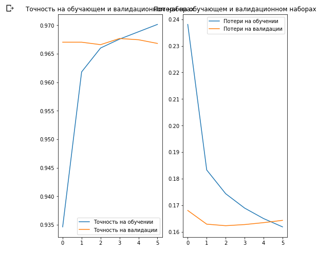
What is interesting here is that the results on the validation dataset are better than the results on the training dataset from the very beginning to the very end of the learning process.

One reason for this behavior is that the accuracy on the validation dataset is measured at the end of the training iteration, and the accuracy on the training dataset is considered as the average of all training iterations.

The biggest reason for this behavior is the use of the pre-trained MobileNet sub-network, which was previously trained on a large data set of cats and dogs. In the learning process, our network continues to expand the input training data set (the same augmentation), but not the validation set. This means that the generated images on the training data set are more difficult to classify than normal images from the validated data set.

Check Prediction Results

To repeat the graph from the previous section, first you need to get a sorted list of class names:

 class_names = np.array(info.features['label'].names) class_names
      
      

        
        
        
      

    
        
        
        
      
      

        
        
        
      

    
     

Output:

 array(['cat', 'dog'], dtype='<U3')
      
      

        
        
        
      

    
        
        
        
      
      

        
        
        
      

    
     

Pass the block with images through the model and convert the resulting indexes into class names:

 predicted_batch = model.predict(image_batch) predicted_batch = tf.squeeze(predicted_batch).numpy() predicted_ids = np.argmax(predicted_batch, axis=-1) predicted_class_names = class_names[predicted_ids] predicted_class_names
      
      

        
        
        
      

    
        
        
        
      
      

        
        
        
      

    
     

Output:

 array(['cat', 'cat', 'cat', 'cat', 'dog', 'cat', 'dog', 'cat', 'cat', 'cat', 'cat', 'cat', 'dog', 'cat', 'cat', 'dog', 'cat', 'cat', 'cat', 'cat', 'cat', 'cat', 'dog', 'dog', 'dog', 'dog', 'cat', 'cat', 'dog', 'cat', 'cat', 'dog'], dtype='<U3')
      
      

        
        
        
      

    
        
        
        
      
      

        
        
        
      

    
     

Let's take a look at the true labels and predicted:

 print(": ", label_batch) print(": ", predicted_ids)
      
      

        
        
        
      

    
        
        
        
      
      

        
        
        
      

    
     

Output:

 : [0 0 0 0 1 0 1 0 0 0 0 0 1 0 0 1 0 0 0 0 0 0 1 1 1 1 0 1 1 0 0 1] : [0 0 0 0 1 0 1 0 0 0 0 0 1 0 0 1 0 0 0 0 0 0 1 1 1 1 0 0 1 0 0 1]
      
      

        
        
        
      

    
        
        
        
      
      

        
        
        
      

    
     

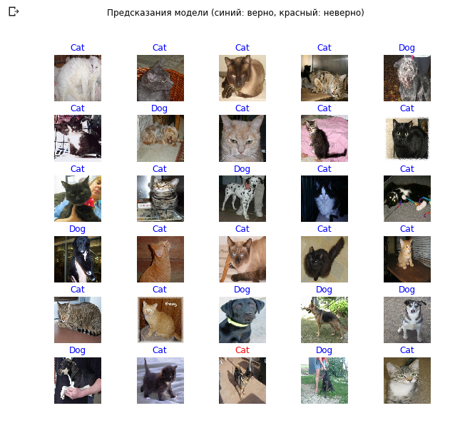
 plt.figure(figsize=(10, 9)) for n in range(30): plt.subplot(6, 5, n+1) plt.subplots_adjust(hspace=0.3) plt.imshow(image_batch[n]) color = "blue" if predicted_ids[n] == label_batch[n] else "red" plt.title(predicted_class_names[n].title(), color=color) plt.axis('off') _ = plt.suptitle("  (: , : )")
      
      

        
        
        
      

    
        
        
        
      
      

        
        
        
      

    
     

Diving into convolutional neural networks

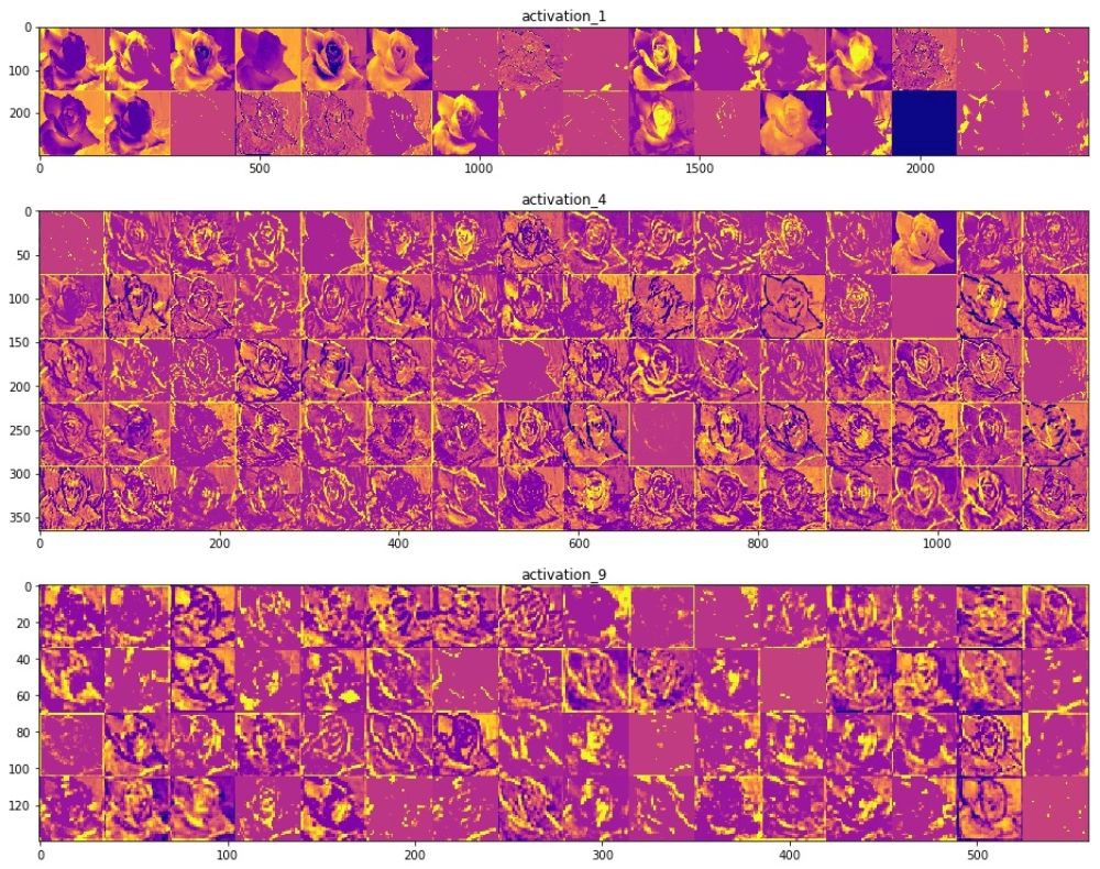
Using convolutional neural networks, we managed to make sure that they cope well with the task of classifying images. However, at the moment, we can hardly imagine how they really work. If we could understand how the learning process takes place, then, in principle, we could improve the classification work even further. One way to understand how convolutional neural networks work is to visualize the layers and the results of their work. We strongly recommend that you study the materials here to better understand how to visualize the results of convolutional layers.

The field of computer vision saw the light at the end of the tunnel and has made significant progress since the advent of convolutional neural networks. The incredible speed with which research in this area is carried out and the huge arrays of images published on the Internet have given incredible results over the past few years. The rise of convolutional neural networks began with AlexNet in 2012, which was created by Alex Krizhevsky, Ilya Sutskever and Jeffrey Hinton and won the famous ImageNet Large-Scale Visual Recognition Challenge. Since then, there was no doubt about the bright future using convolutional neural networks, and the field of computer vision and the results of work in it only confirmed this fact. Starting from recognizing your face on a mobile phone and ending with recognition of objects in autonomous cars, convolutional neural networks have already managed to show and prove their strength and solve many problems from the real world.

Despite the huge number of large data sets and pre-trained models of convolutional neural networks, it is sometimes extremely difficult to understand how the network works and what exactly this network is trained for, especially for people who do not have sufficient knowledge in the field of machine learning. , , , Inception, . . , , , , .

" Python"

François Chollet. , . Keras, , " " TensorFlow, MXNET Theano. , , . , .

, , .

(training accuracy) . , , , , Inception, .

, , . Inception v3 ( ImageNet) , Kaggle. Inception, , Inception v3 .

10 () 32 , 2292293. 0.3195, — 0.6377. ImageDataGenerator



, . GitHub .

, "" , . .

, Inception v3 , .

— . .

, () . (), , , , . , , , , .

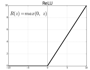
ReLU- . , ReLU(z) = max(0, z)



.

, , , , , , , , .. , . "" () , , , .

"" . .

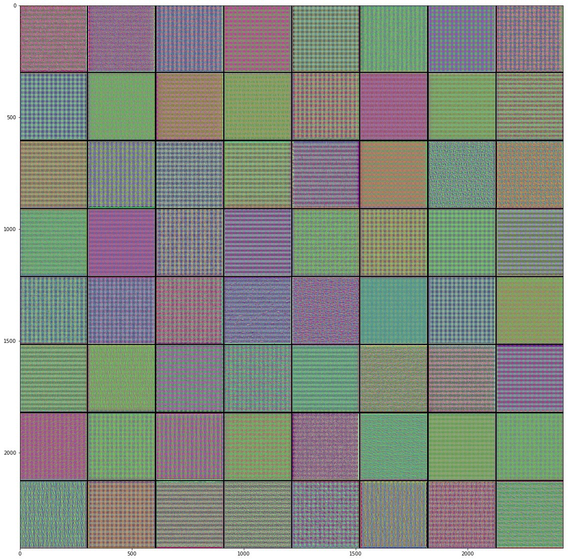
, Inveption V3 :

, . , , , , .. , , . , , , "" ( , ).

, , , . , .

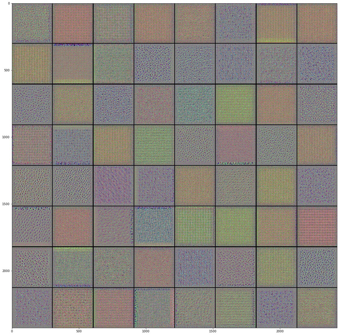
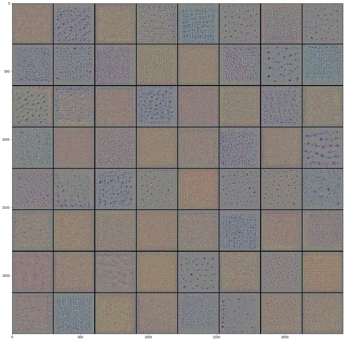
Class Activation Map ( ). CAM . 2D , .

, . , , Mixed- Inception V3-, . () , .

, , . , , . , . , , , , .

, "" - . . .

, , .

:

Colab Colab .

TensorFlow Hub

TensorFlow Hub , .

. , , , .

.

Runtime -> Reset all runtimes...

, :

 from __future__ import absolute_import, division, print_function, unicode_literals import numpy as np import matplotlib.pyplot as plt import tensorflow as tf tf.enable_eager_execution() import tensorflow_hub as hub import tensorflow_datasets as tfds from tensorflow.keras import layers
      
      

        
        
        
      

    
        
        
        
      
      

        
        
        
      

    
     

Output:

 WARNING:tensorflow: The TensorFlow contrib module will not be included in TensorFlow 2.0. For more information, please see: * https://github.com/tensorflow/community/blob/master/rfcs/20180907-contrib-sunset.md * https://github.com/tensorflow/addons * https://github.com/tensorflow/io (for I/O related ops) If you depend on functionality not listed there, please file an issue.
      
      

        
        
        
      

    
        
        
        
      
      

        
        
        
      

    
     

 import logging logger = tf.get_logger() logger.setLevel(logging.ERROR)
      
      

        
        
        
      

    
        
        
        
      
      

        
        
        
      

    
     

TensorFlow Datasets

TensorFlow Datasets. , — tf_flowers



. , . tfds.splits



(70%) (30%). tfds.load



. tfds.load



, , .

 splits = tfds.Split.TRAIN.subsplit([70, 30]) (training_set, validation_set), dataset_info = tfds.load('tf_flowers', with_info=True, as_supervised=True, split=splits)
      
      

        
        
        
      

    
        
        
        
      
      

        
        
        
      

    
     

Output:

 Downloading and preparing dataset tf_flowers (218.21 MiB) to /root/tensorflow_datasets/tf_flowers/1.0.0... Dl Completed... 1/|/100% 1/1 [00:07<00:00, 3.67s/ url] Dl Size... 218/|/100% 218/218 [00:07<00:00, 30.69 MiB/s] Extraction completed... 1/|/100% 1/1 [00:07<00:00, 7.05s/ file] Dataset tf_flowers downloaded and prepared to /root/tensorflow_datasets/tf_flowers/1.0.0. Subsequent calls will reuse this data.
      
      

        
        
        
      

    
        
        
        
      
      

        
        
        
      

    
     

, , () , , — .

 num_classes = dataset_info.features['label'].num_classes num_training_examples = 0 num_validation_examples = 0 for example in training_set: num_training_examples += 1 for example in validation_set: num_validation_examples += 1 print('Total Number of Classes: {}'.format(num_classes)) print('Total Number of Training Images: {}'.format(num_training_examples)) print('Total Number of Validation Images: {} \n'.format(num_validation_examples))
      
      

        
        
        
      

    
        
        
        
      
      

        
        
        
      

    
     

Output:

 Total Number of Classes: 5 Total Number of Training Images: 2590 Total Number of Validation Images: 1080
      
      

        
        
        
      

    
        
        
        
      
      

        
        
        
      

    
     

— .

 for i, example in enumerate(training_set.take(5)): print('Image {} shape: {} label: {}'.format(i+1, example[0].shape, example[1]))
      
      

        
        
        
      

    
        
        
        
      
      

        
        
        
      

    
     

Output:

 Image 1 shape: (226, 240, 3) label: 0 Image 2 shape: (240, 145, 3) label: 2 Image 3 shape: (331, 500, 3) label: 2 Image 4 shape: (240, 320, 3) label: 0 Image 5 shape: (333, 500, 3) label: 1
      
      

        
        
        
      

    
        
        
        
      
      

        
        
        
      

    
     

— , MobilNet v2 — 224224 (grayscale). image



() label



() .

 IMAGE_RES = 224 def format_image(image, label): image = tf.image.resize(image, (IMAGE_RES, IMAGE_RES))/255.0 return image, label BATCH_SIZE = 32 train_batches = training_set.shuffle(num_training_examples//4).map(format_image).batch(BATCH_SIZE).prefetch(1) validation_batches = validation_set.map(format_image).batch(BATCH_SIZE).prefetch(1)
      
      

        
        
        
      

    
        
        
        
      
      

        
        
        
      

    
     

TensorFlow Hub

TensorFlow Hub . , , .

feature_extractor



MobileNet v2. , TensorFlow Hub ( ) . . tf2-preview/mobilenet_v2/feature_vector



, URL MobileNet v2 . feature_extractor



hub.KerasLayer



input_shape



.

 URL = "https://tfhub.dev/google/tf2-preview/mobilenet_v2/feature_vector/4" feature_extractor = hub.KerasLayer(URL, input_shape=(IMAGE_RES, IMAGE_RES, 3))
      
      

        
        
        
      

    
        
        
        
      
      

        
        
        
      

    
     

, :

 feature_extractor.trainable = False
      
      

        
        
        
      

    
        
        
        
      
      

        
        
        
      

    
     

, . . .

 model = tf.keras.Sequential([ feature_extractor, layers.Dense(num_classes, activation='softmax') ]) model.summary()
      
      

        
        
        
      

    
        
        
        
      
      

        
        
        
      

    
     

Output:

 Model: "sequential" _________________________________________________________________ Layer (type) Output Shape Param # ================================================================= keras_layer (KerasLayer) (None, 1280) 2257984 _________________________________________________________________ dense (Dense) (None, 5) 6405 ================================================================= Total params: 2,264,389 Trainable params: 6,405 Non-trainable params: 2,257,984
      
      

        
        
        
      

    
        
        
        
      
      

        
        
        
      

    
     

, .

 model.compile( optimizer='adam', loss='sparse_categorical_crossentropy', metrics=['accuracy']) EPOCHS = 6 history = model.fit(train_batches, epochs=EPOCHS, validation_data=validation_batches)
      
      

        
        
        
      

    
        
        
        
      
      

        
        
        
      

    
     

Output:

 Epoch 1/6 81/81 [==============================] - 17s 216ms/step - loss: 0.7765 - acc: 0.7170 - val_loss: 0.0000e+00 - val_acc: 0.0000e+00 Epoch 2/6 81/81 [==============================] - 12s 147ms/step - loss: 0.3806 - acc: 0.8757 - val_loss: 0.3485 - val_acc: 0.8833 Epoch 3/6 81/81 [==============================] - 12s 146ms/step - loss: 0.3011 - acc: 0.9031 - val_loss: 0.3190 - val_acc: 0.8907 Epoch 4/6 81/81 [==============================] - 12s 147ms/step - loss: 0.2527 - acc: 0.9205 - val_loss: 0.3031 - val_acc: 0.8917 Epoch 5/6 81/81 [==============================] - 12s 148ms/step - loss: 0.2177 - acc: 0.9371 - val_loss: 0.2933 - val_acc: 0.8972 Epoch 6/6 81/81 [==============================] - 12s 146ms/step - loss: 0.1905 - acc: 0.9456 - val_loss: 0.2870 - val_acc: 0.9000
      
      

        
        
        
      

    
        
        
        
      
      

        
        
        
      

    
     

~90% 6 , ! , , ~76% 80 . , MobilNet v2 .

.

 acc = history.history['acc'] val_acc = history.history['val_acc'] loss = history.history['loss'] val_loss = history.history['val_loss'] epochs_range = range(EPOCHS) plt.figure(figsize=(8, 8)) plt.subplot(1, 2, 1) plt.plot(epochs_range, acc, label='Training Accuracy') plt.plot(epochs_range, val_acc, label='Validation Accuracy') plt.legend(loc='lower right') plt.title('Training and Validation Accuracy') plt.subplot(1, 2, 2) plt.plot(epochs_range, loss, label='Training Loss') plt.plot(epochs_range, val_loss, label='Validation Loss') plt.legend(loc='upper right') plt.title('Training and Validation Loss') plt.show()
      
      

        
        
        
      

    
        
        
        
      
      

        
        
        
      

    
     

, , .

, , .

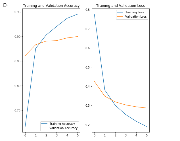
- MobileNet, . ( augmentation), . .

NumPy. , .

 class_names = np.array(dataset_info.features['label'].names) print(class_names)
      
      

        
        
        
      

    
        
        
        
      
      

        
        
        
      

    
     

Output:

 ['dandelion' 'daisy' 'tulips' 'sunflowers' 'roses']
      
      

        
        
        
      

    
        
        
        
      
      

        
        
        
      

    
     

next()



image_batch



( ) label_batch



( ). image_batch



label_batch



NumPy .numpy()



. .predict()



. np.argmax()



. .

 image_batch, label_batch = next(iter(train_batches)) image_batch = image_batch.numpy() label_batch = label_batch.numpy() predicted_batch = model.predict(image_batch) predicted_batch = tf.squeeze(predicted_batch).numpy() predicted_ids = np.argmax(predicted_batch, axis=-1) predicted_class_names = class_names[predicted_ids] print(predicted_class_names)
      
      

        
        
        
      

    
        
        
        
      
      

        
        
        
      

    
     

Output:

 ['sunflowers' 'roses' 'tulips' 'tulips' 'daisy' 'dandelion' 'tulips' 'sunflowers' 'daisy' 'daisy' 'tulips' 'daisy' 'daisy' 'tulips' 'tulips' 'tulips' 'dandelion' 'dandelion' 'tulips' 'tulips' 'dandelion' 'roses' 'daisy' 'daisy' 'dandelion' 'roses' 'daisy' 'tulips' 'dandelion' 'dandelion' 'roses' 'dandelion']
      
      

        
        
        
      

    
        
        
        
      
      

        
        
        
      

    
     

 print("Labels: ", label_batch) print("Predicted labels: ", predicted_ids)
      
      

        
        
        
      

    
        
        
        
      
      

        
        
        
      

    
     

Output:

 Labels: [3 4 2 2 1 0 2 3 1 1 2 1 1 2 2 2 0 0 2 2 0 4 1 1 0 4 1 2 0 0 4 0] Predicted labels: [3 4 2 2 1 0 2 3 1 1 2 1 1 2 2 2 0 0 2 2 0 4 1 1 0 4 1 2 0 0 4 0]
      
      

        
        
        
      

    
        
        
        
      
      

        
        
        
      

    
     

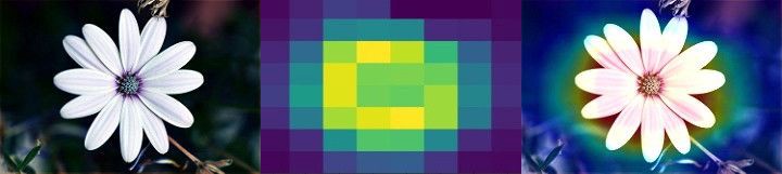
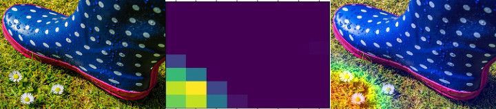
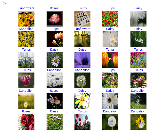
 plt.figure(figsize=(10,9)) for n in range(30): plt.subplot(6,5,n+1) plt.subplots_adjust(hspace = 0.3) plt.imshow(image_batch[n]) color = "blue" if predicted_ids[n] == label_batch[n] else "red" plt.title(predicted_class_names[n].title(), color=color) plt.axis('off') _ = plt.suptitle("Model predictions (blue: correct, red: incorrect)")
      
      

        
        
        
      

    
        
        
        
      
      

        
        
        
      

    
     

Inception-

TensorFlow Hub tf2-preview/inception_v3/feature_vector



. Inception V3 . , Inception V3 . , Inception V3 299299 . Inception V3 MobileNet V2.

 IMAGE_RES = 299 (training_set, validation_set), dataset_info = tfds.load('tf_flowers', with_info=True, as_supervised=True, split=splits) train_batches = training_set.shuffle(num_training_examples//4).map(format_image).batch(BATCH_SIZE).prefetch(1) validation_batches = validation_set.map(format_image).batch(BATCH_SIZE).prefetch(1) URL = "https://tfhub.dev/google/tf2-preview/inception_v3/feature_vector/4" feature_extractor = hub.KerasLayer(URL, input_shape=(IMAGE_RES, IMAGE_RES, 3), trainable=False) model_inception = tf.keras.Sequential([ feature_extractor, tf.keras.layers.Dense(num_classes, activation='softmax') ]) model_inception.summary()
      
      

        
        
        
      

    
        
        
        
      
      

        
        
        
      

    
     

Output:

 Model: "sequential_1" _________________________________________________________________ Layer (type) Output Shape Param # ================================================================= keras_layer_1 (KerasLayer) (None, 2048) 21802784 _________________________________________________________________ dense_1 (Dense) (None, 5) 10245 ================================================================= Total params: 21,813,029 Trainable params: 10,245 Non-trainable params: 21,802,784
      
      

        
        
        
      

    
        
        
        
      
      

        
        
        
      

    
     

 model_inception.compile( optimizer='adam', loss='sparse_categorical_crossentropy', metrics=['accuracy']) EPOCHS = 6 history = model_inception.fit(train_batches, epochs=EPOCHS, validation_data=validation_batches)
      
      

        
        
        
      

    
        
        
        
      
      

        
        
        
      

    
     

Output:

 Epoch 1/6 81/81 [==============================] - 44s 541ms/step - loss: 0.7594 - acc: 0.7309 - val_loss: 0.0000e+00 - val_acc: 0.0000e+00 Epoch 2/6 81/81 [==============================] - 35s 434ms/step - loss: 0.3927 - acc: 0.8772 - val_loss: 0.3945 - val_acc: 0.8657 Epoch 3/6 81/81 [==============================] - 35s 434ms/step - loss: 0.3074 - acc: 0.9120 - val_loss: 0.3586 - val_acc: 0.8769 Epoch 4/6 81/81 [==============================] - 35s 434ms/step - loss: 0.2588 - acc: 0.9282 - val_loss: 0.3385 - val_acc: 0.8796 Epoch 5/6 81/81 [==============================] - 35s 436ms/step - loss: 0.2252 - acc: 0.9375 - val_loss: 0.3256 - val_acc: 0.8824 Epoch 6/6 81/81 [==============================] - 35s 435ms/step - loss: 0.1996 - acc: 0.9440 - val_loss: 0.3164 - val_acc: 0.8861
      
      

        
        
        
      

    
        
        
        
      
      

        
        
        
      

    
     

Summary

. :

• : , . .
• : . "" , , .
• MobileNet: Google, . MobileNet .

MobileNet . . MobileNet .

… call-to-action — , share :)

YouTube

Telegram

In contact with

Ojok .