Model-oriented design. Creation of a reliable model, using an aviation heat exchanger as an example
In a previous article on model-oriented design , it was shown why an object model is needed, and it was proved that without this object model one can speak about model based design only as a marketing blizzard, meaningless and merciless. But when an object model appears, competent engineers always have a reasonable question: what evidence is there that the mathematical model of an object corresponds to a real object.

One example of the answer to this question is given in the article about model-oriented design of the electric drive. In this article we will consider an example of creating a model for aviation air conditioning systems, diluting the practice with some theoretical general considerations.
Creating a reliable model of the object. Theory
In order not to pull the rubber, I’ll immediately tell you about the algorithm for creating a model for model-oriented design. It has only three simple steps:
Step 1. Develop a system of algebraic-differential equations that describe the dynamic behavior of the simulated systems. It is simple if you know the physics of the process. Many scientists have already developed for us the basic physical laws of the name of Newton, Brenuli, Navier Stokes and other Shtangels of Compasses and Rabinovich.
Step 2. In the resulting system, isolate the set of empirical coefficients and characteristics of the simulation object that can be obtained from the tests.
Step 3. Carry out tests of the object and adjust the model according to the results of field experiments, so that it corresponds to reality, with the necessary degree of detail.
As you can see, just exactly two three.
Practical example
The air conditioning system (SCR) in the aircraft is connected to the automatic pressure maintenance system. The pressure in the aircraft should always be greater than the external pressure, while the rate of change in pressure should be such that the pilots and passengers do not bleed nose and ears. Therefore, the control system of the inflow and outflow of air is important for safety, and expensive test systems are put on the ground for its development. They create temperatures and pressures of flight altitude, reproduce take-off and landing modes at airfields of different heights. And the question of developing and debugging control systems for hard currency is rising to its full potential. How long will we drive the test bench to get a satisfactory control system? Obviously, if we set up the control model on the model of the object, then the cycle of work on the test bench can be significantly reduced.
The aviation air conditioning system consists of the same heat exchangers as any other thermal system. Battery - it is also a battery in Africa, only air conditioning. But due to the limitation of the take-off mass and the dimensions of the aircraft, the heat exchangers are made as compact as possible and as efficient as possible in order to transfer as much heat as possible from the lower mass. As a result, the geometry becomes quite bizarre. As for example in the case under consideration. Figure 1 shows a plate heat exchanger, in which a membrane is used between the plates to improve heat transfer. Hot and cold coolant alternate in the channels, while the flow direction is transverse. One coolant is supplied to the frontal cut, the other to the side.
To solve the SCR control problem, we need to know how much heat is transferred from one medium to another in such a heat exchanger per unit time. The rate of change of temperature depends on this, which we regulate.
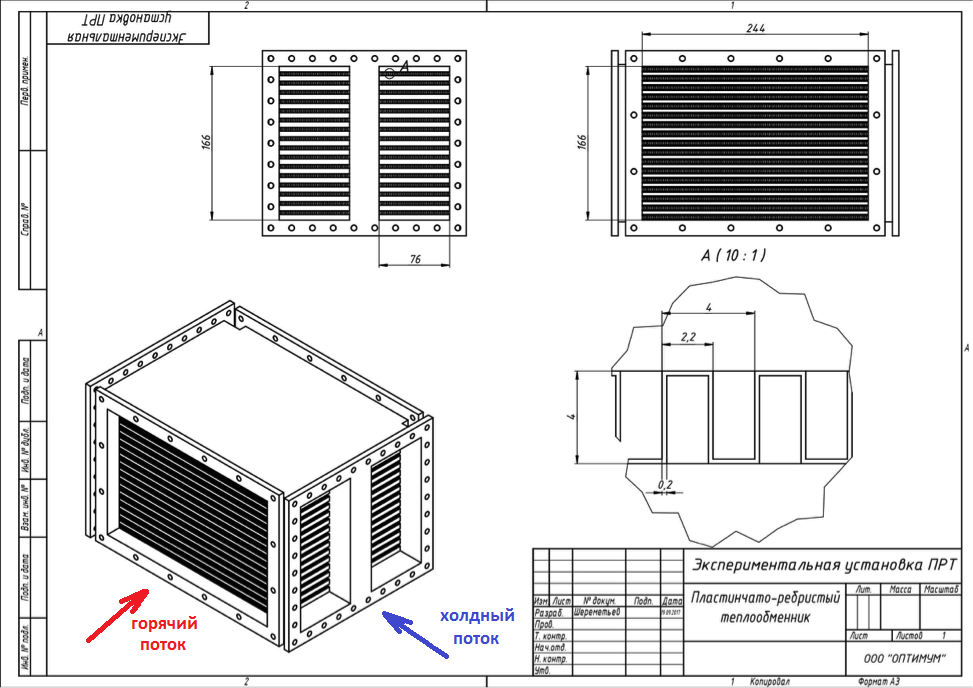
Figure 1. Aircraft heat exchanger diagram.
Modeling problems. Hydraulic part
At first glance, the task is quite simple, it is necessary to calculate the mass flow through the channels of the heat exchanger and the heat flow between the channels.
The mass flow rate of the coolant in the channels is calculated using the Bernoulli formula:

Where:
ΔP is the pressure drop between two points;
ξ is the friction coefficient of the coolant;
L is the length of the channel;
d is the hydraulic diameter of the channel;
ρ is the density of the coolant;
ω is the velocity of the coolant in the channel.
For a channel of arbitrary shape, the hydraulic diameter is calculated by the formula:

Where:
F is the area of the bore;
P - wetted channel perimeter.
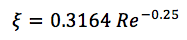
The friction coefficient is calculated by empirical formulas and depends on the flow velocity and the properties of the coolant. For different geometries, different dependencies are obtained, for example, the formula for turbulent flow in smooth pipes:
Where:
Re is the Reynolds number.
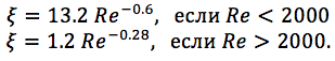
For flow in flat channels, the following formula can be used:
From the Bernoulli formula, you can calculate the pressure drop for a given speed, or vice versa, calculate the velocity of the coolant in the channel, based on a given pressure drop.
Heat exchange
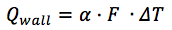
The heat flow between the coolant and the wall is calculated by the formula:
Where:
α [W / (m2 × deg)] - heat transfer coefficient;
F is the area of the bore.
For the problems of flow of coolants in pipes, a sufficient number of studies has been carried out and there are many calculation methods, and as a rule, it all comes down to empirical dependences, for the heat transfer coefficient α [W / (m2 × deg)]
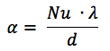
Where:
Nu is the Nusselt number,
λ is the thermal conductivity of the liquid [W / (m × deg)]
d is the hydraulic (equivalent) diameter.
Empirical criteria are used to calculate the Nusselt number (criterion), for example, the formula for calculating the Nusselt number of a round pipe looks like this:
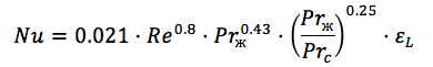
Here we already see the Reynolods number, the Prandtl number at wall temperature and fluid temperature, and the coefficient of unevenness. ( Source )
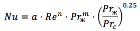
For corrugated plate heat exchangers, the formula is similar ( Source ):
Where:
n = 0.73 m = 0.43 for a turbulent flow,
coefficient a - varies between 0.065 and 0.6, depending on the number of plates and the flow regime.
Note that this coefficient is calculated for only one point in the stream. For the next point, we have a different liquid temperature (it has warmed up or cooled), a different wall temperature and, accordingly, all Reynolds numbers and Prandtl numbers are floating.
At this point, any mathematician will say that it is impossible to calculate exactly a system in which the coefficient changes 10 times, and he will be right.
Any practicing engineer will say that each heat exchanger is different in manufacturing and it is impossible to calculate the system, and it will also be right.
But what about model-oriented design? Is it all gone?
Advanced sellers of Western software in this place will pair you with Supercomputers and 3D-calculation systems, such as "without it in any way." And you need to run the calculation for a day to get the temperature distribution for 1 minute.
It is clear that this is not our option, we need to debug the control system, if not in real time, then at least in the foreseeable future.
Poke method
A heat exchanger is manufactured, a series of tests is carried out, and a table of the efficiency of the steady-state temperature is set at the given flow rates. Simple, fast and reliable, as the data obtained from the tests.
The disadvantage of this approach is that there are no dynamic characteristics of the object. Yes, we know what the steady-state heat flux will be, but we do not know how long it will be established when switching from one operation mode to another.
Therefore, having calculated the necessary characteristics, we set up the control system directly during the tests, which we would like to avoid from the very beginning.
Model Oriented Approach
To create a model of a dynamic heat exchanger, it is necessary to use test data, to eliminate uncertainties in empirical calculation formulas - the Nusselt number and hydraulic resistance.
The decision is simple, like all ingenious. We take the empirical formula, conduct experiments and determine the value of the coefficient a, thereby eliminating the uncertainty in the formula.
As soon as we have a certain value of the heat transfer coefficient, all other parameters are determined by the basic physical laws of conservation. The temperature difference and the heat transfer coefficient determine the amount of energy transmitted to the channel per unit time.
Knowing the energy flow, it is possible to solve the equations of conservation of energy mass and momentum for the coolant in the hydraulic channel. For example, this:
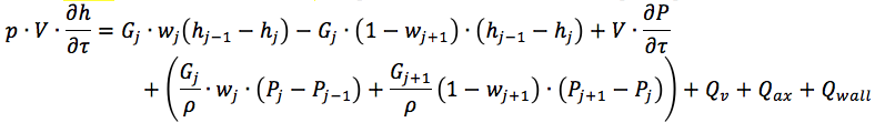
For our case, the heat flux between the wall and the heat carrier - Qwall - remains undetermined. More details can be found here ...
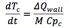
And also the equation of the temperature derivative for the channel wall:
Where:
ΔQ wall - the difference between the incoming and outgoing flow to the channel wall;
M is the mass of the channel wall;
C pc is the heat capacity of the wall material.
Model accuracy
As mentioned above, in the heat exchanger we have a temperature distribution over the surface of the plate. For the steady-state value, one can take the average over the plates and use it, presenting the entire heat exchanger as a single concentrated point, in which heat transfer occurs over the entire surface of the heat exchanger at the same temperature difference. But for transient modes, this approximation may not work. The other extreme is to make several hundred thousand points and load the Super Computer, which also does not suit us, since the task is to configure the control system in real time, or better, faster.
The question arises, how many sections do you need to break the heat exchanger to get acceptable accuracy and speed of calculation?
As always by chance, I had a model of an amine heat exchanger on hand. The heat exchanger is a tube, heating medium flows in the pipes, and heated between the pits. To simplify the task, the entire tube of the heat exchanger can be represented as one equivalent pipe, and the pipe itself can be represented as a set of discrete design cells, in each of which a point model of heat transfer is calculated. The model diagram of a single cell is shown in Figure 2. The hot air channel and the cold air channel are connected through a wall that provides heat transfer between the channels.
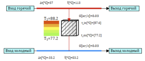
Figure 2. Heat exchanger cell model.
The tubular heat exchanger model is easily customizable. You can change only one parameter - the number of sections along the length of the pipe and look at the calculation results for different partitions. We will calculate several options, starting from dividing into 5 points along the length (Fig. 3) and up to 100 points along the length (Fig. 4).
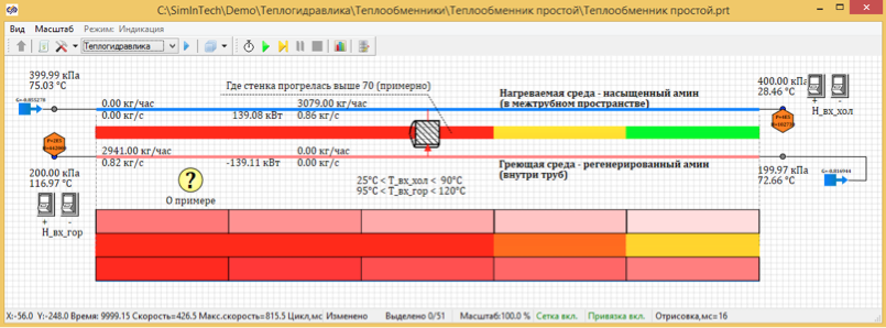
Figure 3. Stationary temperature distribution of 5 design points.
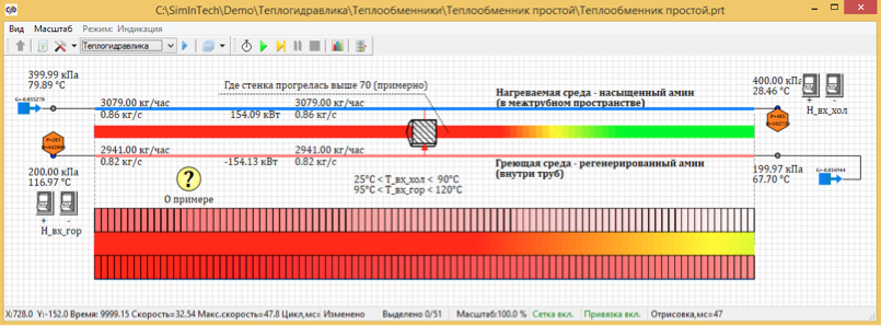
Figure 4. Stationary temperature distribution of 100 design points.
As a result of the calculations, it turned out that the steady-state temperature when divided by 100 points is 67.7 degrees. And when divided into 5 calculated points, the temperature is 72, 66 degrees C.
Also, the calculation speed relative to real time is displayed in the lower part of the window.
Let's see how the steady-state temperature and the calculation speed change depending on the number of design points. The difference in steady-state temperatures in calculations with different numbers of calculated cells can be used to assess the accuracy of the result.
Table 1. The dependence of temperature and calculation speed on the number of design points along the length of the heat exchanger.
| Number of design points | Steady temperature | Calculation speed |
| 5 | 72.66 | 426 |
| 10 | 70.19 | 194 |
| 25 | 68.56 | 124 |
| fifty | 67.99 | 66 |
| one hundred | 67.8 | 32 |
Analyzing this table, we can draw the following conclusions:
- The calculation speed decreases in proportion to the number of design points in the heat exchanger model.
- The change in calculation accuracy occurs exponentially. As the number of points increases, the refinement at each subsequent increase decreases.
In the case of a plate heat exchanger with a cross-flow heat carrier, as in Figure 1, the creation of an equivalent model from elementary design cells is slightly complicated. We need to connect the cells in such a way as to organize the cross-flow. For 4 cells, the circuit will look as shown in Figure 5.
The coolant flow is divided into two channels along the hot and cold branch, the channels will connect through thermal structures, so that when passing through the channel, the coolant exchanges heat with different channels. Simulating the cross-flow, the hot heat carrier flows from left to right (see Fig. 5) in each channel, sequentially exchanging heat with the channels of the cold heat carrier, which goes from the bottom up (see Fig. 5). The hottest point is in the upper left corner, since the hot heat carrier exchanges heat with the already heated coolant of the cold channel. And the coldest in the lower right, where the cold coolant exchanges heat with the hot coolant that has already cooled in the first section.
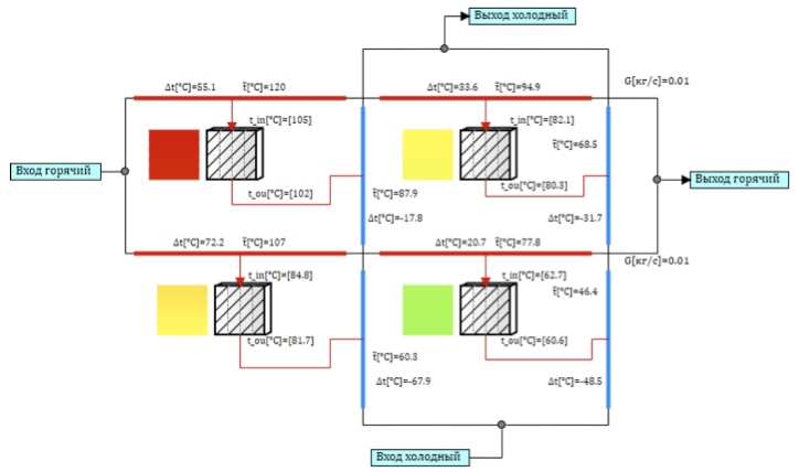
Figure 5. A cross-flow model of 4 design cells.
Such a model for a plate heat exchanger does not take into account the heat transfer between the cells due to thermal conductivity and does not take into account the mixing of the coolant, since each channel is insulated.
But in our case, the latter restriction does not reduce accuracy, since in the design of the heat exchanger, the corrugated membrane divides the flow into many isolated channels along the coolant (see Fig. 1). Let's see what happens with the accuracy of the calculation when modeling a plate heat exchanger with an increase in the number of design cells.
For accuracy analysis, we use two options for dividing the heat exchanger into the design cell:
- Each square cell contains two hydraulic (cold and hot flows) and one thermal element. (see figure 5)
- Each square cell contains six hydraulic elements (three sections in hot and cold flows) and three thermal elements.
In the latter case, we use two types of connection:
- counter flow of cold and hot streams;
- associated flow of cold and hot flow.
The oncoming current increases the efficiency in comparison with the cross-flow, and the associated current decreases. With a large number of cells, flow averaging occurs and everything becomes close to the actual transverse flow around (see Figure 6).
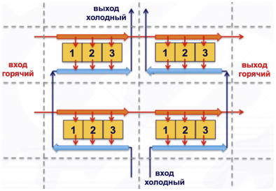
Figure 6. A cross-flow model of four cells with 3 elements.
Figure 7 shows the results of a steady-state stationary temperature distribution in the heat exchanger when air is supplied at a temperature of 150 ° C along the hot line, and 21 ° C along the cold line, for various options for partitioning the model. The color and numbers on the cell reflect the average wall temperature in the cell.
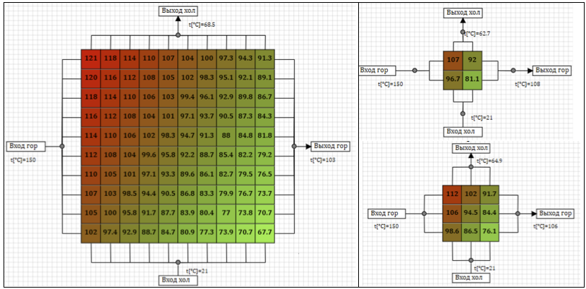
Figure 7. Steady-state temperatures for different calculation schemes.
Table 2 shows the steady-state temperature of the heated air after the heat exchanger, depending on the partition of the heat exchanger model into cells.
Table 2. Temperature dependence on the number of design cells in the heat exchanger.
| Dimension Model | Steady temperature
1 item in a cell | Steady temperature
3 items in a cell |
| 2x2 | 62.7 | 67.7 |
| 3x3 | 64.9 | 68.5 |
| 4x4 | 66.2 | 68.9 |
| 8x8 | 68.1 | 69.5 |
| 10x10 | 68.5 | 69.7 |
| 20x20 | 69.4 | 69.9 |
| 40x40 | 69.8 | 70.1 |
With an increase in the number of computational cells in the model, the final steady-state temperature increases. The difference between the steady-state temperature at different partitions can be considered as an indicator of calculation accuracy. It can be seen that with an increase in the number of calculation cells, the temperature tends to the limit, and the increase in accuracy is not proportional to the number of calculation points.
The question arises, but what accuracy of the model do we need?
The answer to this question depends on the purpose of our model. Since this article is about model-oriented design, we are creating a model for customizing the control system. This means that the accuracy of the model must be comparable with the accuracy of the sensors used in the system.
In our case, the temperature is measured by a thermocouple, in which the accuracy is ± 2.5 ° C. Any accuracy higher for the purpose of tuning the control system is useless, our real control system simply "will not see it." Thus, if we assume that the limit temperature with an infinite number of partitions is 70 ° C, then a model that gives us more than 67.5 ° C will be of sufficient accuracy. All models with 3 points in the calculation cell and models larger than 5x5 with one point in the cell. (Highlighted in green in table 2)
Dynamic operating modes
To assess the dynamic mode, we evaluate the process of temperature change at the hottest and coldest points of the heat exchanger wall for various design schemes. (see fig. 8)
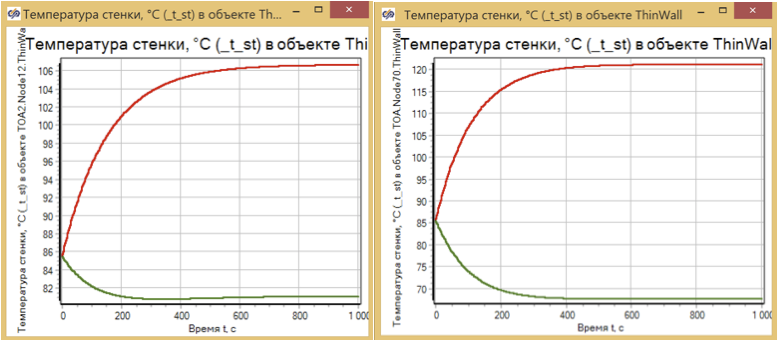
Figure 8. Heat exchanger warming up. Models of dimension 2x2 and 10x10.
It can be seen that the time of the transition process and its very nature, practically do not depend on the number of calculated cells, and are determined solely by the mass of the heated metal.
Thus, we conclude that for honest modeling of the heat exchanger in the modes from 20 to 150 ° C, with the accuracy required by the SCR control system, about 10 - 20 calculated points are enough.
Experiment dynamic model setup
Having a mathematical model, as well as experimental data on the purge of a heat exchanger, it remains for us to make a simple correction, namely, to introduce an intensification coefficient into the model so that the calculation coincides with the experimental results.
Moreover, using the graphical environment for creating the model, we will do this automatically. Figure 9 presents an algorithm for selecting heat transfer intensification coefficients. The data obtained from the experiment are fed to the input, the heat exchanger model is connected, and the necessary coefficients for each of the modes are obtained at the output.
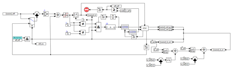
Figure 9. The algorithm for selecting the coefficient of intensification according to the results of the experiment.
Thus, we determine the same coefficient for a Nusselt number and eliminate the uncertainty in the calculation formulas. For different operating modes and temperatures, the values of correction factors can vary, however, for similar operating modes (normal operation), they turn out to be very close. For example, for a given heat exchanger for different modes, the coefficient is from 0.492 to 0.655
If we apply the coefficient 0.6, then in the studied operating modes the calculation error will be less than the error of the thermocouple, thus, for the control system, the mathematical model of the heat exchanger will be fully adequate to the present model.
Heat exchanger model setup results
To assess the quality of heat transfer, a special characteristic is used - efficiency:
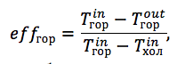
Where:
eff mountains - heat exchanger efficiency for a hot heat carrier;
T mountains in - temperature at the inlet to the heat exchanger along the path of movement of the hot coolant;
T mountains out - temperature at the outlet of their heat exchanger along the path of movement of the hot heat carrier;
T cold in - temperature at the inlet to the heat exchanger along the path of movement of the coolant.
Table 3 shows the values of the deviation of the efficiency of the heat exchanger model from the experimental one at various flows on the hot and cold lines.
Table 3. Errors in calculating heat transfer efficiency in%
In our case, the selected coefficient can be used in all operating modes that we are interested in. If at low flow rates, where the error is greater, the necessary accuracy is not achieved, we can use a variable coefficient of intensification, which will depend on the current flow rate.
For example, in Figure 10, the intensification coefficient is calculated according to a given formula depending on the current flow rate in the channel cells.
Figure 10. Variable heat transfer coefficient.
findings
- Knowledge of physical laws allows you to create dynamic object models for model-oriented design.
- The model must be verified and tuned according to test data.
- Model development tools should allow the developer to customize the model based on the test results of the object.
- Use the right model-oriented approach and you will be happy!
Bonus for those who have read. Video of the virtual model of the hard currency system.
All Articles