The book "Quantum Mechanics. Theoretical minimum "

Classical mechanics is intuitive: it is daily and repeatedly used by people for survival. But until the twentieth century, no one ever used quantum mechanics. She describes things so small that they completely fall out of the human perception of the senses. The only way to understand this theory, to enjoy its beauty, is to block our intuition with abstract mathematics.



Leonard Susskind - the famous American scientist - invites you to go on an exciting journey to the country of quantum mechanics. On the way you will benefit from basic knowledge from the school course of physics, as well as the basics of mathematical analysis and linear algebra. You also need to know something about the issues that were addressed in the first book of the "theoretical minimum" of Susskind - "Everything you need to know about modern physics." But it's okay if this knowledge is somewhat forgotten. Much of the author will remind and explain along the way.



Quantum mechanics is an unusual theory: according to its postulates, for example, we can know everything about the system and nothing about its individual parts. Einstein and Niels Bohr argued a lot about this and other contradictions. If you are not afraid of difficulties, have an inquisitive mind, are technically literate, sincerely and deeply interested in physics, then you will like this course of lectures by Leonard Susskind. The book focuses on the logical principles of quantum theory and aims not to smooth out the paradox of quantum logic, but to pull it out into the daylight and try to deal with the difficult questions that it raises.

Wave function overview

In this lecture, we will use the language of wave functions, so let's do a short review of the material before the dive. We discussed in lecture 5 the wave functions of abstract objects, without explaining how they relate to waves or functions. Before filling this gap, I’ll remind you of what we discussed earlier.



Let us begin by choosing the observable L with eigenvalues ​​l and eigenvectors | l〉. Let | Y be a state vector. Since the eigenvectors of the Hermitian operator form a complete orthonormal basis, the vector | Y〉 can be decomposed into this basis:



As you remember from sections 5.1.2 and 5.1.3, the values ​​of Y (l) are called the wave function of the system. But note: the specific form of Y (l) depends on the particular observable L, which we initially chose. If we choose another observable, the wave function (along with the basis vectors and eigenvalues) will be different, despite the fact that we are still talking about the same state. Thus, we must make the reservation that Y (l) is a wave function associated with | Yñ. To be precise, we must say that Y (l) is a wave function in the L-basis. If we use the properties of the orthonormality of this basis of the vectors 〈li | lj〉 = dij, then the wave function in this L-basis can also be specified using internal products (or projections) of the state vector | Y on the eigenvectors | l〉: Y (l ) = 〈L | Y〉



One can think of the wave function in two ways. First of all, it is a set of components of the state vector in a particular basis. These components can be written in the form of a column vector:







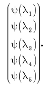
Another way to think about the wave function is to consider it as a function of l. If you specify any valid value for l, then the function Y (l) gives a complex number. Thus, it can be said that Y (l) is a complex-valued function of a discrete variable l. With this consideration, linear operators become operations that apply to functions and provide new functions.



And one last reminder: the probability that the experiment will give the result l is equal to P (l) = Y * (l) Y (l).

Functions and vectors

Until now, the systems we studied had finite-dimensional state vectors. For example, a simple spin is described by a two-dimensional state space. For this reason, the observables had only a finite number of possible observable values. But there are more complex observables that can have an infinite number of values. An example is a particle. The coordinates of a particle are observable, but unlike spin, coordinates have an infinite number of possible values. For example, a particle moving along the x axis can be at any real x mark. In other words, x is a continuous infinite variable. When the observed systems are continuous, the wave function becomes a complete function of a continuous variable. To apply quantum mechanics to systems of this kind, we must expand the concept of vectors so as to include functions in it.



Functions are functions, and vectors are vectors; they seem to be completely different entities, so in what sense are functions as vectors? If you think of vectors as arrows in three-dimensional space, then, of course, they are not at all the same as functions. But if you look at the vectors more broadly, as mathematical objects that satisfy certain postulates, the functions actually form a vector space. This vector space is often called the Hilbert space in honor of the mathematician David Gilbert.



Consider the set of complex functions Y (x) of one real variable x. By a complex function, I mean that to each x it associates a complex number Y (x). On the other hand, the independent variable x is an ordinary real variable. It can take any real values ​​from –∞ to + ∞.



We now formulate exactly what we mean by saying that “functions are vectors”. This is not a superficial analogy or metaphor. Under certain constraints (to which we will return), functions such as Y (x) satisfy the mathematical axioms that define the vector space. We casually mentioned this idea in section 1.9.2, and now we use it in full force. Looking back at the axioms of a complex vector space (in section 1.9.1), we see that complex functions satisfy all of them.



1. The sum of any two functions is a function.

2. The addition of functions is commutative.

3. Addition of functions associatively.

4. There is a unique zero function such that when it is added to any function, the same function is obtained.

5. For any given function Y (x), there is a unique function –Y (x) such that Y (x) + (–Y (x)) = 0.

6. Multiplying a function by any complex number gives a function and is linear.

7. Distribution property is observed, meaning that



z [Y (x) + j (x)] = zY (x) + zj (x),

[z + w] Y (x) = zY (x) + wY (x),



where z and w are complex numbers.



All this implies that we can identify the function Y (x) with the ket vector | Y in the abstract vector space. It is not surprising that we can also define bras-vectors. The sconce vector 〈Y |, corresponding to the ketus | Y〉, is identified with the complex conjugate function Y * (x).



To effectively use this idea, we need to summarize some of the items from our set of mathematical tools. In previous lectures, labels that identified wave functions were members of some finite discrete set, for example, the eigenvalues ​​of a certain observable. But now the independent variable is continuous. Among other things, this means that we cannot summarize it using normal amounts. I think you know what to do. Here are function-oriented substitutes for our three vector concepts, two of which you already know.



• Amounts are replaced by integrals.

• Probabilities are replaced by probability densities.

• The Kronecker delta symbol is replaced by the Dirac delta function.



Take a closer look at these tools.



The sums are replaced by integrals . If we really wanted to maintain severity, we would start by replacing the x axis with a discrete set of points separated by very small ε intervals, and then move to the ε → 0 limit. It would take several pages to justify each step. But we can avoid these troubles with a few intuitive definitions, such as replacing sums with integrals. Schematically, this approach can be written as:







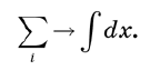
For example, if it is necessary to calculate the area under a curve, the x-axis is divided into tiny segments, then the areas of a large number of rectangles are added, exactly as is done in elementary mathematical analysis. When we let the segments shrink to zero, the sum becomes an integral.



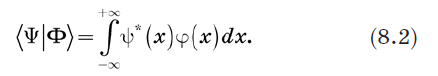
Consider a bra 〈Y | and ket | Y〉 and define their inner product. An obvious way to do this is to replace the summation in equation (1.2) with integration. We define the inner product as:







Probabilities are replaced by probability densities . Next, we identify P (x) = Y * (x) Y (x) with the probability density for the variable x. Why precisely with the density of probability, and not just with probability? If x is a continuous variable, then the probability that it will accept any exactly specified value is usually zero. Therefore, it is more correct to put the question this way: what is the probability that x lies between two values ​​x = a and x = b? The probability density is determined so that this probability is given by the integral







Since the total probability must be 1, we can define the vector normalization as







The Kronecker delta symbol is replaced by the Dirac delta function . Until now, everything was very familiar. Dirac's delta function is something new. The delta function is analogous to the Kronecker delta symbol dij, which by definition is equal to 0 if i ≠ j, and 1 if i = j. But it can be defined in a different way. Consider any vector Fi in a finite-dimensional space. It is easy to see that the Kronecker delta symbol satisfies the condition







This is due to the fact that in this sum only the members with j = i are non-zero. During the summation, the Kronecker symbol filters out all the components of F except Fi. An obvious generalization of this is to define a new function that has the same filtering property when used under the integral. In other words, we need a new entity d (x - x '), which has the property that for any function F (x)







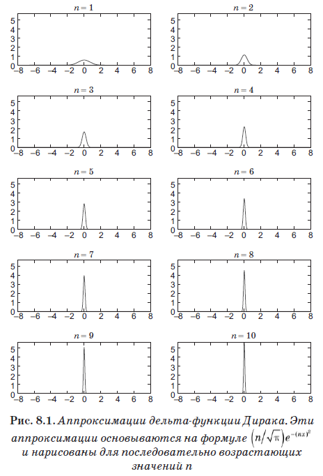
Equation (8.4) defines a new entity called the Dirac delta function, which turned out to be the most important tool in quantum mechanics. But despite its name, it is not really a function in the usual sense. It is zero where x ≠ x ', but when x = x' it goes to infinity. In fact, it is infinite just so that the area under d (x) is equal to 1. Roughly speaking, this function is non-zero on an infinitely small interval ε, but on this interval it has a value of 1 / ε. Thus, the area under it is 1, and, more importantly, it satisfies equation (8.4). Function







fairly well approximates the delta function for very large values ​​of n. In fig. Figure 8.1 shows this optimization with increasing values ​​of n. Despite the fact that we stopped at n = 10, that is, a very small value, note that the schedule has already become a very narrow and sharp peak.







»More information about the book can be found on the publisher's website.

» Table of Contents

» Excerpt



For readers of this blog 20% ​​discount coupon - Susskind