使用されるライブラリのほとんどはすでにAnaconda 3ディストリビューションに含まれているため、使用することをお勧めします。 欠落しているモジュール/ライブラリは、pip install“ package name”を介して標準としてインストールできます。
次のライブラリを接続します。
import numpy as np import pandas as pd import nltk import re import os import codecs from sklearn import feature_extraction import mpld3 import matplotlib.pyplot as plt import matplotlib as mpl
分析のために、任意のデータを取得できます。 このタスクは、私の目に留まりました: 国家支出プロジェクトの検索クエリの統計 。 データを3つのグループに分割する必要がありました:民間、州、および商業組織。 私は特別なものを発明したくなかったので、この場合にクラスタリングがどのようにつながるかを確認することにしました(実際にはそうではありませんが)。 ただし、一部の一般のVKからデータをダウンロードできます。
import vk # id session = vk.Session(access_token='') # URL access_token, tvoi_id id : # https://oauth.vk.com/authorize?client_id=tvoi_id&scope=friends,pages,groups,offline&redirect_uri=https://oauth.vk.com/blank.html&display=page&v=5.21&response_type=token api = vk.API(session) poss=[] id_pab=-59229916 #id , id info=api.wall.get(owner_id=id_pab, offset=0, count=1) kolvo = (info[0]//100)+1 shag=100 sdvig=0 h=0 import time while h<kolvo: if(h>70): print(h) # , pubpost=api.wall.get(owner_id=id_pab, offset=sdvig, count=100) i=1 while i < len(pubpost): b=pubpost[i]['text'] poss.append(b) i=i+1 h=h+1 sdvig=sdvig+shag time.sleep(1) len(poss) import io with io.open("public.txt", 'w', encoding='utf-8', errors='ignore') as file: for line in poss: file.write("%s\n" % line) file.close() titles = open('public.txt', encoding='utf-8', errors='ignore').read().split('\n') print(str(len(titles)) + ' ') import re posti=[] # for line in titles: chis = re.sub(r'(\<(/?[^>]+)>)', ' ', line) #chis = re.sub() chis = re.sub('[^-- ]', '', chis) posti.append(chis)
検索クエリデータを使用して、短いテキストデータがどの程度クラスター化されていないかを示します。 以前にテキストから特殊文字と句読点を削除し、略語を置き換えました(たとえば、SPは個人の起業家です)。 テキストが判明しました。各行には1つの検索クエリがありました。
データを配列に読み込み、正規化に進みます-単語を最初の形式に縮小します。 これは、Porter Stemmer、MyStem Stemmer、PyMorphy2を使用していくつかの方法で実行できます。 警告します-MyStemはラッパーを介して動作するため、操作の速度は非常に遅くなります。 ポーターステマーについて説明しますが、他のユーザーを他のユーザーと組み合わせて使用することはありません(たとえば、PyMorphy2を経由して、ポーターステマーを実行するなど)。
titles = open('material4.csv', 'r', encoding='utf-8', errors='ignore').read().split('\n') print(str(len(titles)) + ' ') from nltk.stem.snowball import SnowballStemmer stemmer = SnowballStemmer("russian") def token_and_stem(text): tokens = [word for sent in nltk.sent_tokenize(text) for word in nltk.word_tokenize(sent)] filtered_tokens = [] for token in tokens: if re.search('[--]', token): filtered_tokens.append(token) stems = [stemmer.stem(t) for t in filtered_tokens] return stems def token_only(text): tokens = [word.lower() for sent in nltk.sent_tokenize(text) for word in nltk.word_tokenize(sent)] filtered_tokens = [] for token in tokens: if re.search('[--]', token): filtered_tokens.append(token) return filtered_tokens # () totalvocab_stem = [] totalvocab_token = [] for i in titles: allwords_stemmed = token_and_stem(i) #print(allwords_stemmed) totalvocab_stem.extend(allwords_stemmed) allwords_tokenized = token_only(i) totalvocab_token.extend(allwords_tokenized)
Pymorphy2
import pymorphy2 morph = pymorphy2.MorphAnalyzer() G=[] for i in titles: h=i.split(' ') #print(h) s='' for k in h: #print(k) p = morph.parse(k)[0].normal_form #print(p) s+=' ' s += p #print(s) #G.append(p) #print(s) G.append(s) pymof = open('pymof_pod.txt', 'w', encoding='utf-8', errors='ignore') pymofcsv = open('pymofcsv_pod.csv', 'w', encoding='utf-8', errors='ignore') for item in G: pymof.write("%s\n" % item) pymofcsv.write("%s\n" % item) pymof.close() pymofcsv.close()
pymystem3
ライブラリを初めて使用するときに、現在のオペレーティングシステムのアナライザー実行可能ファイルが自動的にダウンロードおよびインストールされます。
from pymystem3 import Mystem m = Mystem() A = [] for i in titles: #print(i) lemmas = m.lemmatize(i) A.append(lemmas) # "" import pickle with open("mystem.pkl", 'wb') as handle: pickle.dump(A, handle)
TF-IDF重み行列を作成します。 各検索クエリをドキュメントと見なします(これは、各ツイートがドキュメントであるTwitterの投稿を分析するときに行われます)。 sklearnパッケージからtfidf_vectorizerを取得し、ntlkパッケージからストップワードを取得します(最初はnltk.download()でダウンロードする必要があります)。 パラメータは、適切なように調整できます-上限と下限からn-gramの数まで(この場合は3を取ります)。
stopwords = nltk.corpus.stopwords.words('russian') # - stopwords.extend(['', '', '', '', '', '', '', '', '']) from sklearn.feature_extraction.text import TfidfVectorizer, CountVectorizer n_featur=200000 tfidf_vectorizer = TfidfVectorizer(max_df=0.8, max_features=10000, min_df=0.01, stop_words=stopwords, use_idf=True, tokenizer=token_and_stem, ngram_range=(1,3)) get_ipython().magic('time tfidf_matrix = tfidf_vectorizer.fit_transform(titles)') print(tfidf_matrix.shape)
結果のマトリックス上で、さまざまなクラスタリング手法の適用を開始します。
num_clusters = 5 # - - KMeans from sklearn.cluster import KMeans km = KMeans(n_clusters=num_clusters) get_ipython().magic('time km.fit(tfidf_matrix)') idx = km.fit(tfidf_matrix) clusters = km.labels_.tolist() print(clusters) print (km.labels_) # MiniBatchKMeans from sklearn.cluster import MiniBatchKMeans mbk = MiniBatchKMeans(init='random', n_clusters=num_clusters) #(init='k-means++', 'random' or an ndarray) mbk.fit_transform(tfidf_matrix) %time mbk.fit(tfidf_matrix) miniclusters = mbk.labels_.tolist() print (mbk.labels_) # DBSCAN from sklearn.cluster import DBSCAN get_ipython().magic('time db = DBSCAN(eps=0.3, min_samples=10).fit(tfidf_matrix)') labels = db.labels_ labels.shape print(labels) # from sklearn.cluster import AgglomerativeClustering agglo1 = AgglomerativeClustering(n_clusters=num_clusters, affinity='euclidean') #affinity : cosine, l1, l2, manhattan get_ipython().magic('time answer = agglo1.fit_predict(tfidf_matrix.toarray())') answer.shape
受信したデータをデータフレームにグループ化し、各クラスターに分類されるリクエストの数を計算できます。
#k-means clusterkm = km.labels_.tolist() #minikmeans clustermbk = mbk.labels_.tolist() #dbscan clusters3 = labels #agglo #clusters4 = answer.tolist() frame = pd.DataFrame(titles, index = [clusterkm]) #k-means out = { 'title': titles, 'cluster': clusterkm } frame1 = pd.DataFrame(out, index = [clusterkm], columns = ['title', 'cluster']) #mini out = { 'title': titles, 'cluster': clustermbk } frame_minik = pd.DataFrame(out, index = [clustermbk], columns = ['title', 'cluster']) frame1['cluster'].value_counts() frame_minik['cluster'].value_counts()
クエリの数が多いため、テーブルを見るのはあまり便利ではなく、理解のためにインタラクティブ性を高めたいと考えています。 したがって、リクエストの相対的な相対的な位置のグラフを作成します。
最初に、ベクトル間の距離を計算する必要があります。 このために、コサイン距離が使用されます。 記事では、負の値がなく、0から1の範囲になるように、1からの減算を使用することを提案しています。
from sklearn.metrics.pairwise import cosine_similarity dist = 1 - cosine_similarity(tfidf_matrix) dist.shape
グラフは2次元と3次元になり、元の距離行列はn次元になるため、次元削減アルゴリズムを使用する必要があります。 (MDS、PCA、t-SNE)から選択する多くのアルゴリズムがありますが、インクリメンタルPCAで停止しましょう。 この選択は、実用的なアプリケーションの結果として行われました-MDSとPCAを試しましたが、十分なRAM(8ギガバイト)がなく、スワップファイルが使用され始めたときに、すぐにコンピューターを再起動することができました。
インクリメンタルPCAアルゴリズムは、分解されるデータセットが大きすぎてRAMに収まらない場合に、主成分法(PCA)の代わりとして使用されます。 IPCAは、入力データサンプルの数に依存しないメモリサイズを使用して、入力の低レベルの近似値を作成します。
# - PCA from sklearn.decomposition import IncrementalPCA icpa = IncrementalPCA(n_components=2, batch_size=16) get_ipython().magic('time icpa.fit(dist) #demo =') get_ipython().magic('time demo2 = icpa.transform(dist)') xs, ys = demo2[:, 0], demo2[:, 1] # PCA 3D from sklearn.decomposition import IncrementalPCA icpa = IncrementalPCA(n_components=3, batch_size=16) get_ipython().magic('time icpa.fit(dist) #demo =') get_ipython().magic('time ddd = icpa.transform(dist)') xs, ys, zs = ddd[:, 0], ddd[:, 1], ddd[:, 2] # , #from mpl_toolkits.mplot3d import Axes3D #fig = plt.figure() #ax = fig.add_subplot(111, projection='3d') #ax.scatter(xs, ys, zs) #ax.set_xlabel('X') #ax.set_ylabel('Y') #ax.set_zlabel('Z') #plt.show()
視覚化自体に直接進みます。
from matplotlib import rc # font = {'family' : 'Verdana'}#, 'weigth': 'normal'} rc('font', **font) # import random def generate_colors(n): color_list = [] for c in range(0,n): r = lambda: random.randint(0,255) color_list.append( '#%02X%02X%02X' % (r(),r(),r()) ) return color_list # cluster_colors = {0: '#ff0000', 1: '#ff0066', 2: '#ff0099', 3: '#ff00cc', 4: '#ff00ff',} # , - 01234 cluster_names = {0: '0', 1: '1', 2: '2', 3: '3', 4: '4',} #matplotlib inline # data frame, ( PCA) + df = pd.DataFrame(dict(x=xs, y=ys, label=clusterkm, title=titles)) # groups = df.groupby('label') fig, ax = plt.subplots(figsize=(72, 36)) #figsize for name, group in groups: ax.plot(group.x, group.y, marker='o', linestyle='', ms=12, label=cluster_names[name], color=cluster_colors[name], mec='none') ax.set_aspect('auto') ax.tick_params( axis= 'x', which='both', bottom='off', top='off', labelbottom='off') ax.tick_params( axis= 'y', which='both', left='off', top='off', labelleft='off') ax.legend(numpoints=1) # 1 # / , #for i in range(len(df)): # ax.text(df.ix[i]['x'], df.ix[i]['y'], df.ix[i]['title'], size=6) # plt.show() plt.close()
名前を追加して行のコメントを解除すると、次のようになります。
10個のクラスターの例 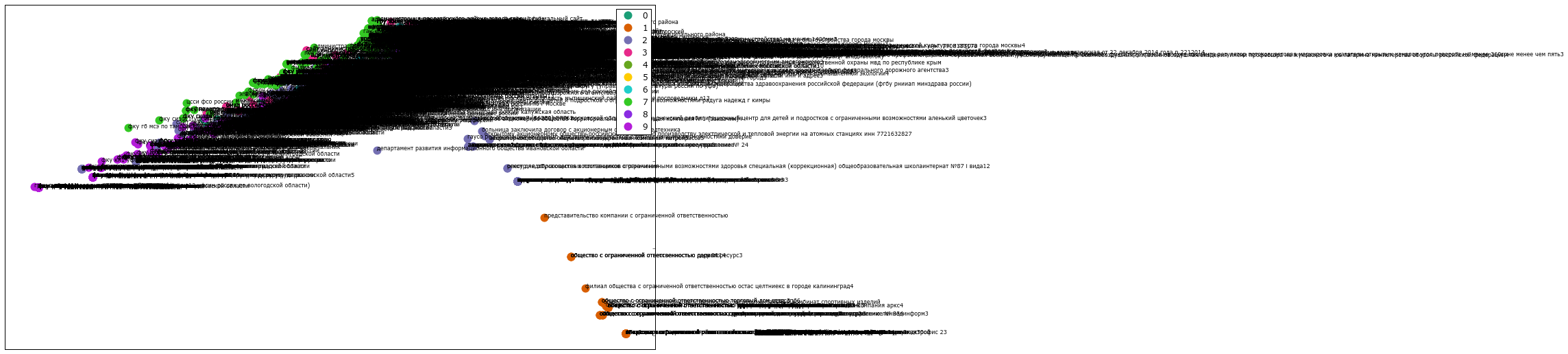
私が期待するようなものではありません。 mpld3を使用して、図面をインタラクティブなグラフに変換します。
# Plot fig, ax = plt.subplots(figsize=(25,27)) ax.margins(0.03) for name, group in groups_mbk: points = ax.plot(group.x, group.y, marker='o', linestyle='', ms=12, #ms=18 label=cluster_names[name], mec='none', color=cluster_colors[name]) ax.set_aspect('auto') labels = [i for i in group.title] tooltip = mpld3.plugins.PointHTMLTooltip(points[0], labels, voffset=10, hoffset=10, #css=css) mpld3.plugins.connect(fig, tooltip) # , TopToolbar() ax.axes.get_xaxis().set_ticks([]) ax.axes.get_yaxis().set_ticks([]) #ax.axes.get_xaxis().set_visible(False) #ax.axes.get_yaxis().set_visible(False) ax.set_title("Mini K-Means", size=20) #groups_mbk ax.legend(numpoints=1) mpld3.disable_notebook() #mpld3.display() mpld3.save_html(fig, "mbk.html") mpld3.show() #mpld3.save_json(fig, "vivod.json") #mpld3.fig_to_html(fig) fig, ax = plt.subplots(figsize=(51,25)) scatter = ax.scatter(np.random.normal(size=N), np.random.normal(size=N), c=np.random.random(size=N), s=1000 * np.random.random(size=N), alpha=0.3, cmap=plt.cm.jet) ax.grid(color='white', linestyle='solid') ax.set_title("", size=20) fig, ax = plt.subplots(figsize=(51,25)) labels = ['point {0}'.format(i + 1) for i in range(N)] tooltip = mpld3.plugins.PointLabelTooltip(scatter, labels=labels) mpld3.plugins.connect(fig, tooltip) mpld3.show()fig, ax = plt.subplots(figsize=(72,36)) for name, group in groups: points = ax.plot(group.x, group.y, marker='o', linestyle='', ms=18, label=cluster_names[name], mec='none', color=cluster_colors[name]) ax.set_aspect('auto') labels = [i for i in group.title] tooltip = mpld3.plugins.PointLabelTooltip(points, labels=labels) mpld3.plugins.connect(fig, tooltip) ax.set_title("K-means", size=20) mpld3.display()
グラフ内の任意のポイントにカーソルを合わせると、対応する検索クエリとともにテキストがポップアップ表示されます。 完成したhtmlファイルの例は次の場所にあります: Mini K-Means
3Dでzoomが必要な場合は、 Plotlyサービスがあり、Python用のプラグインがあります。
Plotly 3D
# 3D import plotly plotly.__version__ import plotly.plotly as py import plotly.graph_objs as go trace1 = go.Scatter3d( x=xs, y=ys, z=zs, mode='markers', marker=dict( size=12, line=dict( color='rgba(217, 217, 217, 0.14)', width=0.5 ), opacity=0.8 ) ) data = [trace1] layout = go.Layout( margin=dict( l=0, r=0, b=0, t=0 ) ) fig = go.Figure(data=data, layout=layout) py.iplot(fig, filename='cluster-3d-plot')
結果は次のとおりです。 例
そして最後のポイントは、ワード方式に従って階層的(凝集的)クラスタリングを実行して、系統樹を作成することです。
In [44]: from scipy.cluster.hierarchy import ward, dendrogram linkage_matrix = ward(dist) fig, ax = plt.subplots(figsize=(15, 20)) ax = dendrogram(linkage_matrix, orientation="right", labels=titles); plt.tick_params(\ axis= 'x', which='both', bottom='off', top='off', labelbottom='off') plt.tight_layout() # plt.savefig('ward_clusters2.png', dpi=200)
結論
残念ながら、自然言語の研究の分野では多くの未解決の問題があり、すべてのデータが特定のグループにグループ化するのが簡単で簡単ではありません。 しかし、このガイドがこのトピックへの関心を高め、さらなる実験の基礎となることを願っています。
すべてのコードは、 https : //github.com/OlegBezverhii/python-notebooks/blob/master/ClasteringRus.pyで入手できます。