
Wolframのディレクター、Michael TrottによるO Tannenbaumのブログの翻訳| Alpha。
このノートブックは、 16世紀のドイツの歌O Tannenbaum (英語版はO Christmas Tree )の音楽の声に合わせて枝を動かす装飾クリスマスツリーのアニメーションを作成する方法を説明しています。 ツリーの選択された枝の1つが指揮者として機能し、ろうそくが指揮者の棒になります。 これにより、すべての節でアニメーションが興味深いものになります。 また、曲の後半に雪と楽しい木の動きを追加します。 最終的なデザインを確認するには、YouTubeで次のビデオをご覧ください。

次の手順を使用してアニメーションを実装します。
- 曲がった枝でクリスマスツリーを構築します。枝は上下左右にスムーズに移動できます。
- 枝に装飾(色の付いたボール、五point星)と異なる色のキャンドルを追加します。 ブランチの終端に対して装飾を移動できます。
- 音の周波数に基づいて、4つの音楽の声を2Dモーションに変換します。 音楽に合わせて指揮者の動きをシミュレートします。
- 強制球面振り子の形の宝石の動きをシミュレートします。 レイリー散逸関数を使用した装飾品の摩擦の説明。
- ホワイトクリスマスに雪を追加します。
- 音楽に関してトゥイーンアニメーションを作成します。
音楽を選択および分析してツリーの動きのデータを取得してくれた同僚のAndrew Steichacherに特に感謝します(以下の「音楽から動きへ」のセクションを参照)。 アニメーションフレームと音楽を1つのビデオクリップに変えてくれたAmy Youngに感謝します。
クリスマスツリー作り
ツリーオプション
木のサイズ、一般的な木の形、枝の数。 変数名はその意味を明らかにします。
(* radial branch count *) radialBranchCount = 3; (* vertical branch count *) verticalBranchCount = 5; (* tree height *) treeHeight = 12; (* tree width *) treeWidth = 6; (* plot points for the B-spline surfaces forming the branches *) {μ, ν} = {6, 8};
幹と枝の色。
stemColor = Directive[Darker[Brown], Lighting -> "Neutral", Specularity[Brown, 20]]; branchTopColor = RGBColor[0., 0.6, 0.6]; branchBottomColor = RGBColor[0., 0.4, 0.4]; branchSideColor = RGBColor[0.4, 0.8, 0.];
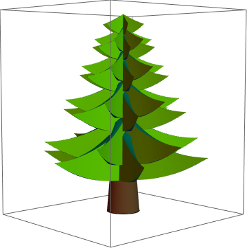
動く木の枝を作る
各ブランチには、さまざまな寸法の(トランクからの距離に応じて)長方形の断面があります。 枝の先端が少し上を向くようにして、見慣れたクリスマスツリーの外観にします。 最も広いサイズでは、枝は円錐(トランク)の近くにあります。 変数τは枝先の上下を、変数σは左右の位置を決定します。 Bスプラインの4つのサーフェス(上、下、左、右)からブランチを作成して、サーフェスを定義する少数のポイントで滑らかな外観にします。
branchTopBottom[ tp_, {hb_, ht_}, {φ1_, φ2_}, {rb_, rt_}, R_, {σ_, τ_}] := Module[{A = -0.6, β = 1/2, φm, Pm, dirR, dirφ, r, P1, P, \[ScriptN], \[ScriptP], x, y, ω, ℛ, ξ, \[ScriptH]s, \[ScriptH]}, φm = Mean[{φ1, φ2}]; Pm = R {Cos[φm], Sin[φm]}; dirR = 1. {Cos[φm], Sin[φm]}; dirφ = Reverse[dirR] {-1, 1}; r = If[tp == "top", rt, rb]; (* move cross section radially away from the stem and contract it *) Table[P1 = {r Cos[φ], r Sin[φ]}; Table[P = P1 + s/ν (Pm - P1); \[ScriptN] = dirφ.P; \[ScriptP] = dirR.P; {x, y} = \[ScriptN] Cos[ s/ν Pi/2]^2 dirφ + \[ScriptP] dirR; ω = σ* 1. s/ν Abs[φ2 - φ1]/ radialBranchCount; ℛ = {{Cos[ω], Sin[ω]}, {-Sin[ω], Cos[ω]}}; {x, y} = ℛ.{x, y}; ξ = R s/ν; \[ScriptH]s = {ht, hb} + {ξ (AR (R - ξ) - (hb - ht) (β - 1) ξ), (ht - hb) ξ^2 β}/R^2; \[ScriptH] = If[tp == "top", \[ScriptH]s[[1]], \[ScriptH]s[[2]]] ; {x, y, \[ScriptH] + τ s/ν (ht - hb)}, {s, 0, ν}], {φ, φ1, φ2, (φ2 - φ1)/μ}] // N ]
高さhの半径は、バレルの最大半径と上部の半径0の線形補間にすぎません。
stemRadius[h_, H_] := (H - h)/H
枝の側面は、上面と下面の間の接続要素のみです。
branchOnStem[{{hb_, ht_}, {φ1_, φ2_}, R_}, {τ_, σ_}] := Module[{tBranch, bBranch, sideBranches}, {bBranch, tBranch} = Table[branchTopBottom[p, {hb, ht}, {φ1, φ2}, stemRadius[{hb, ht}, treeHeight], R, {τ, σ}], {p, {"top", "bottom"}}]; sideBranches = Table[BSplineSurface[{tBranch[[j]], bBranch[[j]]}], {j, {1, -1}}]; {branchTopColor, BSplineSurface[tBranch], branchBottomColor, BSplineSurface[bBranch], branchSideColor, sideBranches} ]
将来の使用のために、ブランチの終わりの位置に対してのみ関数を定義しましょう。
branchOnStemEndPoint[ {{hb_, ht_}, {φ1_, φ2_}, R_}, {σ_, τ_}] := Module[{A = -0.6, β = 1/2, Pm, dirR, dirφ, P, \[ScriptN], \[ScriptP], x, y, ω, ξ, \[ScriptH]s, \[ScriptH], φ = φ1, φm = Mean[{φ1, φ2}]}, Pm = R {Cos[φm], Sin[φm]}; dirR = {Cos[φm], Sin[φm]}; {x, y} = dirR.Pm dirR; ω = 1. σ Abs[φ2 - φ1]/radialBranchCount; {x, y} = {{Cos[ω], Sin[ω]}, {-Sin[ω], Cos[ω]}}.{x, y}; \[ScriptH]s = {ht, hb} + (ht - hb) {β - 1., 1}; {x, y, \[ScriptH]s[[1]] + τ (ht - hb)} ]
ブランチとその終端が{σ、τ}の関数として移動できるようにするインタラクティブなデモ。
Manipulate[ Graphics3D[{branchOnStem[{{0, 1}, {Pi/2 - 1/2, Pi/2 + 1/2}, 1 + ρ}, στ], Red, Sphere[branchOnStemEndPoint[{{0, 1}, {Pi/2 - 1/2, Pi/2 + 1/2}, 1 + ρ}, στ], 0.05]}, PlotRange -> {{-2, 2}, {0, 4}, {-1, 2}}, ViewPoint -> {3.17, 0.85, 0.79}], {{ρ, 1.6, "branch length"}, 0, 2, ImageSize -> Small}, {{στ, {0, 0}, "branch\nleft/right\nup/down"}, {-1, -1}, {1, 1}}, ControlPlacement -> Left, SaveDefinitions -> True]

トランクにブランチを追加する
幹はちょうど円錐形で、その上部は木の上部です。
stem = Cone[{{0, 0, 0}, {0, 0, treeHeight}}, 1];
枝のサイズは高さとともに減少し、幾何学的に小さくなります。 すべてのブランチレベルの総数は、ツリーの高さから下のステップの部分を引いたものに等しくなります。
heightList1 = Module[{α = 0.8, hs, sol}, hs = Prepend[Table[C α^k, {k, 0, verticalBranchCount - 1}], 0]; sol = Solve[Total[hs] == 10, C, Reals]; Accumulate[hs /. sol[[1]]]]
{0、2.97477、5.35459、7.25845、8.78153、10.}
treeWidthOfHeight[h_] := treeWidth (treeHeight - h)/treeHeight
枝は隙間なくトランクにぴったりと収まります。
Graphics3D[{{stemColor, stem}, {Darker[Green], Table[Table[ branchOnStem[{2 + heightList1[[{j, j + 1}]], {k , k + 1} 2 Pi/ radialBranchCount , treeWidthOfHeight[Mean[heightList1[[{j, j + 1}]]]]}, {0, 0}], {k, 0, 1}] , {j, 1, verticalBranchCount}]}}, ViewPoint -> {2.48, -2.28, 0.28}]

Graphics3D[{{stemColor, stem}, {Darker[Green], Table[Table[ branchOnStem[{2 + heightList1[[{j, j + 1}]], {k , k + 1} 2 Pi/ radialBranchCount , treeWidthOfHeight[Mean[heightList1[[{j, j + 1}]]]]}, {0, 0}], {k, 0, radialBranchCount - 1}] , {j, 1, verticalBranchCount}]}}, ViewPoint -> {2.48, -2.28, 0.28}]

枝を移動して、よりリアルなツリー形状を取得できます。 これは、今後使用するツリーです。 ツリーのパラメータを変更して別のツリーを使用するのは非常に簡単です。
heightList2 = {2/3, 1/3}.# & /@ Partition[heightList1, 2, 1]; Graphics3D[{{Darker[Brown], stem}, {EdgeForm[], Table[ Table[branchOnStem[ {2 + heightList1[[{j, j + 1}]], {k , k + 1} 2 Pi/ radialBranchCount , treeWidthOfHeight[Mean[heightList1[[{j, j + 1}]]]]}, {0, 0}], {k, 0, radialBranchCount - 1}] , {j, 1, verticalBranchCount}], Table[Table[ branchOnStem[{2 + heightList2[[{j, j + 1}]], {k , k + 1} 2 Pi/ radialBranchCount + Pi/radialBranchCount, treeWidthOfHeight[Mean[heightList2[[{j, j + 1}]]]]}, {0, 0}], {k, 0, radialBranchCount - 1}] , {j, 1, verticalBranchCount - 1}]}}, ViewPoint -> {2.48, -2.28, 0.28}]

枝を増やして木をさらに密にするのは簡単です。
Graphics3D[{{Darker[Brown], stem}, {EdgeForm[], Table[Table[branchOnStem[ {2 + heightList1[[{j, j + 1}]], {k , k + 1} 2 Pi/(2 radialBranchCount) , treeWidthOfHeight[Mean[heightList1[[{j, j + 1}]]]]}, {0, 0}], {k, 0, (2 radialBranchCount) - 1}] , {j, 1, verticalBranchCount}], Table[Table[branchOnStem[{2 + heightList2[[{j, j + 1}]], {k , k + 1} 2 Pi/(2 radialBranchCount) + Pi/(2 radialBranchCount), treeWidthOfHeight[Mean[heightList2[[{j, j + 1}]]]]}, {0, 0}], {k, 0, 2 radialBranchCount - 1}] , {j, 1, verticalBranchCount - 1}]}}, ViewPoint -> {2.48, -2.28, 0.28}]
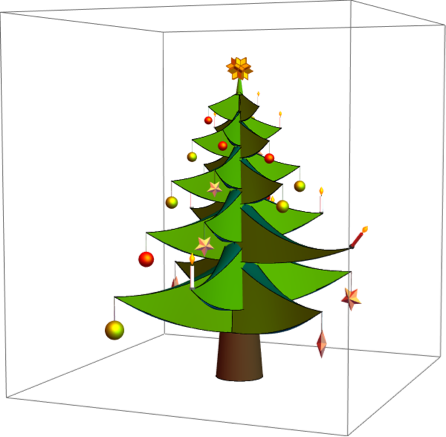
木の飾り
それでは、装飾を作成して、美しく装飾されたクリスマスツリーを作成しましょう。 光沢のあるボール、五point星、キャンドルを追加します。 クリスマスツリーには、オリジナルのチューリンゲンのラウシュボールをお勧めします。 ( ここで見つけることができます)
デコレーション、キャンドル、トップ
カラーボール
各ツリーには、光沢のあるガラス球、おもちゃが必要です。
coloredBall[p_, size_, color_, {ϕ_, θ_}] := Module[{\[ScriptD] = {Cos[ϕ] Sin[θ], Sin[ϕ] Sin[θ], -Cos[θ]}}, {EdgeForm[], GrayLevel[0.4], Specularity[Yellow, 20], Cylinder[{p, p + 1.5 size \[ScriptD]}, 0.02 size ], color, Specularity[Yellow, 10], Sphere[p + (1.5 size + 0.6 size) \[ScriptD] , 0.6 size] }] Graphics3D[{coloredBall[{1, 2, 3}, 1, Red, {0, 0}], coloredBall[{3, 2, 3}, 1, Darker[Blue], {1, 0.2}]}, Axes -> True]

branchOnStemWithBall[{{hb_, ht_}, {φ1_, φ2_}, R_}, {σ_, τ_}, color_, {ϕ_, θ_}] := {branchOnStem[{{hb, ht}, {φ1, φ2}, R}, {σ, τ}] , coloredBall[ branchOnStemEndPoint[{{hb, ht}, {φ1, φ2}, R}, {σ, τ}], 0.45 (ht - hb)/2, color, {ϕ, θ}]}
これはおもちゃのある枝です。 変数{σ、τ}を使用すると、枝の先端に対するボールの位置を変更できます。
Manipulate[ Graphics3D[{branchOnStemWithBall[{{0, 1}, {Pi/2 - 1/2, Pi/2 + 1/2}, 1 + ρ}, στ, Red, ϕθ]}, PlotRange -> {{-2, 2}, {0, 4}, {-2, 2}}, ViewPoint -> {3.17, 0.85, 0.79}], {{ρ, 1.6, "branch length"}, 0, 2, ImageSize -> Small}, {{στ, {0.6, 0.26}, "branch\nleft/right\nup/down"}, {-1, -1}, {1, 1}}, {{ϕθ, {2.57, 1.88}, "ball angles"}, {0, -Pi}, {Pi, Pi}}, ControlPlacement -> Left, SaveDefinitions -> True]

これは、ボールがほとんどまっすぐに垂れ下がっているツリーです。 ボールにランダムな色を使用します。
Graphics3D[{{Darker[Brown], stem}, {Table[ Table[branchOnStemWithBall[{2 + heightList1[[{j, j + 1}]], {k , k + 1} 2 Pi/ radialBranchCount , treeWidthOfHeight[Mean[heightList1[[{j, j + 1}]]]]}, {0, 0}, RandomColor[], {0, 0}], {k, 0, radialBranchCount - 1}] , {j, 1, verticalBranchCount}] }}, ViewPoint -> {2.48, -2.28, 0.28}, Axes -> True]

ランダムな方向にボールを持つツリー。 後で枝を移動する場合、ボールの自然な動きを計算します(つまり、対応する運動方程式を解くことを意味します)。
Graphics3D[{{Darker[Brown], stem}, {Table[ Table[branchOnStemWithBall[{2 + heightList1[[{j, j + 1}]], {k , k + 1} 2 Pi/ radialBranchCount , treeWidthOfHeight[Mean[heightList1[[{j, j + 1}]]]]}, {0, 0}, RandomColor[], {RandomReal[{-Pi, Pi}], RandomReal[{0, Pi}]}], {k, 0, radialBranchCount - 1}] , {j, 1, verticalBranchCount}]}}, ViewPoint -> {2.48, -2.28, 0.28}, Axes -> True]

五point星
次に、いくつかの五point星を作成します。 このオーナメントには回転対称性がないので、私はそれが掛かるスレッドに対して方向角を認めます。
coloredFiveStar[p_, size_, dir_, color_, α_, {ϕ_, θ_}] := Module[{\[ScriptD] = {Cos[ϕ] Sin[θ], Sin[ϕ] Sin[θ], -Cos[θ]}, points, P1, P2, d1, d2, d3, dP, dP2}, d2 = Normalize[dir - dir.\[ScriptD] \[ScriptD]]; d3 = Cross[\[ScriptD], d2]; {EdgeForm[], GrayLevel[0.4], Specularity[Pink, 20], Cylinder[{p, p + (1.5 size + 0.6 size) \[ScriptD]}, 0.02 size ], color, Specularity[Hue[.125], 5], dP = Sin[α] d2 + Cos[α] d3; dP2 = Cross[\[ScriptD], dP]; points = Table[p + (1.5 size + 0.6 size) \[ScriptD] + size If[EvenQ[j], 1, 1/2] * (Cos[j 2 Pi/10 ] \[ScriptD] + Sin[j 2 Pi/10] dP), {j, 0, 10}]; P1 = p + (1.5 size + 0.6 size) \[ScriptD] + size/3 dP2; P2 = p + (1.5 size + 0.6 size) \[ScriptD] - size/3 dP2; {P1, P2} = (p + (1.5 size + 0.6 size) \[ScriptD] + # size/ 3 dP2) & /@ {+1, -1}; Polygon[ Join @@ (Function[a, Append[#, a] & /@ Partition[points, 2, 1]] /@ {P1, P2})] }] Graphics3D[{coloredFiveStar[{1, 2, 3}, 0.2, {0, -1, 0}, Darker[Red], 0, {0, 0}], coloredFiveStar[{1.5, 2, 3}, 0.2, {0, -1, 0}, Darker[Purple], Pi/3, {1, 0.4}]}]

branchOnStemWithFiveStar[{{hb_, ht_}, {φ1_, φ2_}, R_}, {σ_, τ_}, color_, α_, {ϕ_, θ_}] := Module[{dir = Append[Normalize[ Mean[{{Cos[φ1], Sin[φ1]}, {Cos[φ2], Sin[φ2]}}]], 0]}, {branchOnStem[{{hb, ht}, {φ1, φ2}, R}, {σ, τ}] , coloredFiveStar[ branchOnStemEndPoint[{{hb, ht}, {φ1, φ2}, R}, {σ, τ}], 0.4 (ht - hb)/2, dir, color, α, {ϕ, θ}]} ]
木は五point星で飾られています。
Graphics3D[{{Darker[Brown], stem}, {Table[ Table[branchOnStemWithFiveStar[{2 + heightList1[[{j, j + 1}]], {k , k + 1} 2 Pi/ radialBranchCount , treeWidthOfHeight[Mean[heightList1[[{j, j + 1}]]]]}, {0, 0}, RandomColor[], RandomReal[{-Pi, Pi}], {RandomReal[{-Pi, Pi}], RandomReal[0.1 {-1, 1}]}], {k, 0, radialBranchCount - 1}] , {j, 1, verticalBranchCount}] }}, ViewPoint -> {2.48, -2.28, 0.28}, Axes -> True]

ろうそく
私たちは、枝の端に取り付けられた脚から始めて、芯と火で黒くなったワックスのような体でそれらを構築します。 アニメーションを容易にし、火を避けるために、電気キャンドルを使用して、枝が移動しても炎が変わらないようにします。
flamePoints = Table[{0.2 Sin[Pi z]^2 Cos[φ], 0.2 Sin[Pi z]^2 Sin[φ], z}, {z, 0, 1, 1/1/12}, {φ, Pi/2, 5/2 Pi, 2 Pi/24}] litCandle[p_, size_, color_] := {EdgeForm[], color, Cylinder[{p + {0, 0, size 0.001}, p + {0, 0, size 0.5}}, size 0.04], GrayLevel[0.1], Specularity[Orange, 20], Cylinder[{p, p + {0, 0, size 0.05}}, size 0.06], Black, Glow[Black], Cylinder[{ p + {0, 0, size 0.5}, p + {0, 0, size 0.5 + 0.05 size}}, size 0.008], Glow[Orange], Specularity[Hue[.125], 5], BSplineSurface[ Map[(p + {0, 0, size 0.5} + 0.3 size #) &, flamePoints, {2}], SplineClosed -> {True, False}] }
白と赤のキャンドル。
Graphics3D[{litCandle[{0, 0, 0}, 1, Directive[White, Glow[GrayLevel[0.3]], Specularity[Yellow, 20]]], litCandle[{0.5, 0, 0}, 1, Directive[Red, Glow[GrayLevel[0.1]], Specularity[Yellow, 20]]]}]

後でキャンドルの付いた細長い枝を使用して導体にするため、キャンドルを枝から曲げます。
branchOnStemWithCandle[{{hb_, ht_}, {φ1_, φ2_}, R_}, {σ_, τ_}, color_, α_] := {branchOnStem[{{hb, ht}, {φ1, φ2}, R}, {σ, τ}] , If[α == 0, litCandle[ branchOnStemEndPoint[{{hb, ht}, {φ1, φ2}, 0.98 R}, {σ, τ}], 0.66 (ht - hb) , color], Module[{P = branchOnStemEndPoint[{{hb, ht}, {φ1, φ2}, 0.98 R}, {σ, τ}], dir}, dir = Append[Reverse[Take[P, 2]] {-1, 1}, 0]; Rotate[ litCandle[ branchOnStemEndPoint[{{hb, ht}, {φ1, φ2}, 0.98 R}, {σ, τ}], 0.66 (ht - hb) , color], α, dir, P]]]} Manipulate[ Graphics3D[{branchOnStemWithCandle[{{0, 1}, {Pi/2 - 1/2, Pi/2 + 1/2}, 1 + ρ}, στ, Red, α]}, PlotRange -> {{-2, 2}, {0, 4}, {-2, 2}}, ViewPoint -> {3.17, 0.85, 0.79}], {{ρ, 1.6, "branch length"}, 0, 2, ImageSize -> Small}, {{στ, {0, 0}, "branch\nleft/right\nup/down"}, {-1, -1}, {1, 1}}, {{α, Pi/4, "candle angle"}, -Pi, Pi}, ControlPlacement -> Left, SaveDefinitions -> True]
そして、各枝にろうそくを付けたトウヒの木です。
Graphics3D[{{Darker[Brown], stem}, {Table[ Table[branchOnStemWithCandle[{2 + heightList1[[{j, j + 1}]], {k , k + 1} 2 Pi/ radialBranchCount , treeWidthOfHeight[Mean[heightList1[[{j, j + 1}]]]]}, {0, 0}, White, 0], {k, 0, radialBranchCount - 1}] , {j, 1, verticalBranchCount}] }}, ViewPoint -> {2.48, -2.28, 0.28}, Axes -> True]

木のてっぺん
完全な喜びのために、回転交連を上に追加します。
spikey = Cases[ N@Entity["Polyhedron", "RhombicHexecontahedron"][ "Image"], _GraphicsComplex, ∞][[1]]; top = {Gray, Specularity[Red, 25], Cone[{{0, 0, 0.9 treeHeight}, {0, 0, 1.08 treeHeight}}, treeWidth/240], Orange, EdgeForm[Darker[Orange]], Specularity[Hue[.125], 5], MapAt[((0.24 # + {0, 0, 1.08 treeHeight}) & /@ #) &, spikey, 1] } Graphics3D[{{Darker[Brown], stem}, {Table[ Table[branchOnStem[{2 + heightList1[[{j, j + 1}]], {k , k + 1} 2 Pi/ radialBranchCount , treeWidthOfHeight[Mean[heightList1[[{j, j + 1}]]]]}, {0, 0} ], {k, 0, radialBranchCount - 1}] , {j, 1, verticalBranchCount}], top}}, ViewPoint -> {2.48, -2.28, 0.28}, Axes -> True]

木の飾り
1つのブランチをコンダクターとして選択します。 残りの枝をランダムに4つのグループに分け、2色のおもちゃ、五point星、キャンドルで飾ります。
次に、各木の枝に装飾やキャンドルを追加しましょう。 上記のツリーと27のブランチを使用します。 幹の高さと方位角で枝を開始します。
allBranches = Flatten[Riffle[ Table[Table[{2 + heightList1[[{j, j + 1}]], {k , k + 1} 2. Pi/ radialBranchCount , treeWidthOfHeight[Mean[heightList1[[{j, j + 1}]]]]}, {k, 0, radialBranchCount - 1}] , {j, 1, verticalBranchCount}], Table[Table[{2 + heightList2[[{j, j + 1}]], {k , k + 1} 2. Pi/ radialBranchCount + Pi/radialBranchCount, treeWidthOfHeight[Mean[heightList2[[{j, j + 1}]]]]}, {k, 0, radialBranchCount - 1}] , {j, 1, verticalBranchCount - 1}]], 1] Length[allBranches]
27
枝を順番に色付けします。下から赤、上から紫まで順番に色を付けます。
Graphics3D[{{Darker[Brown], stem}, MapIndexed[(branchOnStem[#1, {0, 0}] /. _RGBColor :> Hue[#2[[1]]/36]) &, allBranches], top}, ViewPoint -> {2, 1, -0.2}]

すべてのブランチを音声用の4つのグループとコンダクターの役割用の1つのグループに分けます。
conductorBranch = 7; SeedRandom[12]; voiceBranches = (Last /@ #) & /@ GroupBy[{RandomChoice[{1, 2, 3, 4}], #} & /@ Delete[Range[27], {conductorBranch}], First]
<| 1-> {1、4、5、6、12、18、20}、3-> {2、8、10、11、14、22、23、25}、2-> {3、13 15、16、21、26}、4-> {9、17、19、24、27} |>
voiceBranches = <|1 -> {2, 9, 14, 17, 19, 24, 27}, 2 -> {3, 13, 15, 16, 21, 26}, 3 -> {1, 4, 5, 12, 18, 20}, 4 -> {6, 8, 10, 11, 22, 23, 25}|>
<| 1-> {2、9、14、17、19、24、27}、2-> {3、13、15、16、21、26}、3-> {1、4、5、12 18、20}、4-> {6、8、10、11、22、23、25} |>
以下は、枝が表す声に従って描かれた枝の図です。
Graphics3D[{{Darker[Brown], stem}, branchOnStem[#1, {0, 0}] & /@ allBranches[[voiceBranches[[1]]]] /. _RGBColor :> Yellow, branchOnStem[#1, {0, 0}] & /@ allBranches[[voiceBranches[[2]]]] /. _RGBColor :> White, branchOnStem[#1, {0, 0}] & /@ allBranches[[voiceBranches[[3]]]] /. _RGBColor :> LightBlue, branchOnStem[#1, {0, 0}] & /@ allBranches[[voiceBranches[[4]]]] /. _RGBColor :> Pink, branchOnStem[ allBranches[[conductorBranch]] {1, 1, 1.5}, {0, 0}] /. _RGBColor :> Red, top}, ViewPoint -> {2, 1, -0.2}]

パラメータとしてブランチの終わりの場所を含む完成したツリー。 また、枝の先端の装飾が斜めに座ってカラフルになるようにします。
christmasTree[{{σ1_, τ1_}, {σ2_, τ2_}, {σ3_, τ3_}, {σ4_, τ4_}, {σc_, τc_}}, {{ϕ1_, θ1_}, {ϕ2_, θ2_}, {ϕ3_, θ3_}}, {colBall1_, colBall2_, col5Star_}, conductorEnhancementFactor : fc_, conductorCandleAngle : ωc_, topRotationAngle : ω_] := {{Darker[Brown], stem}, branchOnStemWithBall[#, {σ1, τ1}, colBall1, {ϕ1, θ1}] & /@ allBranches[[voiceBranches[[1]]]], branchOnStemWithBall[#, {σ2, τ2}, colBall2, {ϕ2, θ2}] & /@ allBranches[[voiceBranches[[2]]]], branchOnStemWithFiveStar[#, {σ3, τ3}, col5Star, Pi/4, {ϕ3, θ3}] & /@ allBranches[[voiceBranches[[3]]]], branchOnStemWithCandle[#, {σ4, τ4}, Directive[White, Glow[GrayLevel[0.3]], Specularity[Yellow, 20]], 0] & /@ allBranches[[voiceBranches[[4]]]], branchOnStemWithCandle[ allBranches[[conductorBranch]] {1, 1, 1 + fc}, {σc, τc}, Directive[Red, Glow[GrayLevel[0.1]], Specularity[Yellow, 20]], ωc], Rotate[top, ω, {0, 0, 1}] };
彼女のキャンドルが傾いているすべての枝と細長い導体枝の開始位置。
Graphics3D[christmasTree[{{0, 0}, {0, 0}, {0, 0}, {0, 0}, {0, 0}}, {{0, 0}, {0,0}, {0, 0}}, {Red, Darker[Yellow], Pink}, 0.8, Pi/4, 0], ImageSize -> 600, ViewPoint -> {3.06, 1.28, 0.27}, PlotRange -> {{-7, 7}, {-7, 7}, {0, 15}}]
すべてのパラメーターがランダムに選択された3つのトウヒの木。
SeedRandom[1] Table[Graphics3D[christmasTree[RandomReal[1.5 {-1, 1}, {5, 2}], Table[{RandomReal[{-Pi, Pi}], RandomReal[{0, Pi}]}, 3], RandomColor[3], RandomReal[], RandomReal[Pi/2], 0], ImageSize -> 200, ViewPoint -> {3.06, 1.28, 0.27}, PlotRange -> {{-7, 7}, {-7, 7}, {-2, 15}}], {3}] // Row

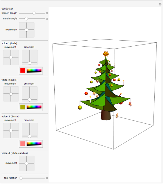
次のインタラクティブデモでは、ブランチを移動したり、ブランチエンドの周りに装飾を移動したり、好きなように装飾を色付けしたりできます。
Manipulate[ Graphics3D[ christmasTree[{στ1, στ2, στ3, στ4, στc}, {ϕθ1, ϕθ2, ϕθ3}, {col1, col2, col3}, l, ωc, ω], ImageSize -> 400, ViewPoint -> {2.61, 1.99, 0.80}, PlotRange -> {{-7, 7}, {-7, 7}, {-2, 15}}], "conductor", {{l, 0.6, "branch length"}, 0, 1, ImageSize -> Small}, {{ωc, Pi/4, "candle angle"}, 0, Pi, ImageSize -> Small}, {{στc, {0, 0}, "movement"}, {-1, -1}, {1, 1}, ImageSize -> Small}, Delimiter, "voice 1 (balls)", Grid[{{"movement", "ornament"}, {Control[{{στ1, {0, 0}, ""}, {-1, -1}, {1, 1}, ImageSize -> Small}], Control[{{ϕθ1, {0, 0}, ""}, {-Pi, 0}, {Pi, Pi}, ImageSize -> Small}]}}], {{col1, Red, ""}, Red, ImageSize -> Tiny}, Delimiter, "voice 2 (balls)", Grid[{{"movement", "ornament"}, {Control[{{στ2, {0, 0}, ""}, {-1, -1}, {1, 1}, ImageSize -> Small}], Control[{{ϕθ2, {0, 0}, ""}, {-Pi, 0}, {Pi, Pi}, ImageSize -> Small}]}}], {{col2, Darker[Yellow], ""}, Red, ImageSize -> Tiny}, Delimiter, "voice 3 (5-star)", Grid[{{"movement", "ornament"}, {Control[{{στ3, {0, 0}, ""}, {-1, -1}, {1, 1}, ImageSize -> Small}], Control[{{ϕθ3, {0, 0}, ""}, {-Pi, 0}, {Pi, Pi}, ImageSize -> Small}]}}], {{col3, Pink, ""}, Red, ImageSize -> Tiny}, Delimiter, "voice 4 (white candles)", Control[{{στ4, {0, 0}, "movement"}, {-1, -1}, {1, 1}, ImageSize -> Small}], Delimiter, Delimiter, {{ω, 0, "top rotation"}, 0, 1, ImageSize -> Small}, ControlPlacement -> Left, SaveDefinitions -> True]
音楽から動きへ
ですから、動く枝と装飾でパラメータ化されたクリスマスツリーを作成し終えたので、枝の動きに対する音楽の比率(そして、装飾)に対処する必要があります。
音のような4つの声を得る
曲のMIDIファイルを使用します。

{ohTannenBaum // Head, ohTannenBaum // ByteCount}
{サウンド、287816}
4票を獲得します。
voices = AssociationThread[{"Soprano", "Alto", "Tenor", "Bass"}, ImportString[ ExportString[ohTannenBaum, "MIDI"], {"MIDI", "SoundNotes"}]]; Sound[Take[#, 10]] & /@ voices

声の頻度
frequencyRules = <|"A1" -> 55., "A2" -> 110., "A3" -> 220., "A4" -> 440., "B1" -> 61.74, "B2" -> 123.5, "B3" -> 246.9, "B4" -> 493.9, "C2" -> 65.41, "C3" -> 130.8, "C4" -> 261.6, "C5" -> 523.3, "D2" -> 73.42, "D#4" -> 311.13, "D4" -> 293.7, "D5" -> 587.3, "E2" -> 82.41, "E4" -> 329.6, "E5" -> 659.3, "F#2" -> 92.50, "F#4" -> 370.0, "G2" -> 98.00, "G#4" -> 415.3, "G4" -> 392.0|>; {minf, maxf} = MinMax[frequencyRules]
{55.、659.3}
最初の投票のタイムライン。
pw[t_] = Piecewise[{frequencyRules[#1], #2[[1]] <= t <= #2[[2]]} & @@@ voices[[1]]]; Plot[pw[t], {t, 0, 100}, PlotRange -> {200, All}, Filling -> Axis, PlotLabel -> "Soprano", Frame -> True, FrameLabel -> {"time in sec", "frequency in Hz"}, AxesOrigin -> {0, 200}]

動きの周波数を表すために、曲線を滑らかにします。
spline = BSplineFunction[Table[{t, pw[t]}, {t, 0, 100, 0.5}], SplineDegree -> 2]

ParametricPlot[spline[t], {t, 0, 100}, AspectRatio -> 0.5, PlotPoints -> 1000]

tMax = 100; Do[ With[{j = j}, pwf[j][t_] = Piecewise[{frequencyRules[#1], #2[[1]] <= t <= #2[[2]]} & @@@ voices[[j]]]; splineFunction[j] = BSplineFunction[Table[{t, pwf[j][t]}, {t, 0, 100, 0.5}], SplineDegree -> 2]; voiceFunction[j][t_Real] := If[0 < t < tMax, splineFunction[j][t/tMax][[2]]/maxf, 0]], {j, 4}]
4つの声の周波数。
Plot[Evaluate[Reverse@Table[pwf[j][t], {j, 4}]], {t, 0, 100}, Frame -> True, FrameLabel -> {"time in sec", "frequency in Hz"}, AspectRatio -> 0.3]

4つの音声の平滑化された周波数。
Plot[Evaluate[Table[voiceFunction[j][t], {j, 4}]], {t, 0, 100}, Frame -> True, FrameLabel -> {"time in sec", "scaled frequency"}, AspectRatio -> 0.3]

これは、3Dでの(平滑化された)最初の3つの音声のグラフです。
ParametricPlot3D[{voiceFunction[1][t], voiceFunction[2][t], voiceFunction[3][t]}, {t, 0, 100}, AspectRatio -> Automatic, PlotPoints -> 1000, BoxRatios -> {1, 1, 1}]

Show[% /. Line[pts_] :> Tube[pts, 0.002], Method -> {"TubePoints" -> 4}]

振動のパターンを取得する
特定のフレーズにスナップして、すべてのビートビートを作成します。
{firstBeat, secondBeat, lastBeat} = voices["Soprano"][[{1, 2, -1}, 2, 1]]
{1.33522、2.00568、98.7727}
anchorDataOChristmasTree = SequenceCases[ voices["Soprano"], (* pattern for "O Christmas Tree, O Christmas Tree..." *) { SoundNote["D4", {pickupStart_, _}, "Trumpet", ___], SoundNote["G4", {beatOne_, _}, "Trumpet", ___], SoundNote["G4", {_, _}, "Trumpet", ___], SoundNote["G4", {beatTwo_, _}, "Trumpet", ___], SoundNote["A4", {beatThree_, _}, "Trumpet", ___], SoundNote["B4", {beatFour_, _}, "Trumpet", ___], SoundNote["B4", {_, _}, "Trumpet", ___], SoundNote["B4", {beatFive_, _}, "Trumpet", ___] } :> <| "PhraseName" -> "O Christmas Tree", "PickupBeat" -> pickupStart, "TargetMeasureBeats" -> {beatOne, beatTwo, beatThree}, "BeatLength" -> Mean@Differences[{pickupStart, beatOne, beatTwo, beatThree, beatFour, beatFive}] |> ]; anchorDataYourBoughsSoGreen = SequenceCases[ voices["Soprano"], (* "Your boughs so green in summertime..." *) { SoundNote["D5", {pickupBeatAnd_, _}, "Trumpet", ___], SoundNote["D5", {beatOne_, _}, "Trumpet", ___], SoundNote["B4", {_, _}, "Trumpet", ___], SoundNote["E5", {beatTwo_, _}, "Trumpet", ___], SoundNote["D5", {beatThreeAnd_, _}, "Trumpet", ___], SoundNote["D5", {beatFour_, _}, "Trumpet", ___], SoundNote["C5", {_, _}, "Trumpet", ___], SoundNote["C5", {beatFive_, _}, "Trumpet", ___] } :> With[ { (* the offbeat nature of this phrase requires some manual work to get things lined up in terms of actual beats *) pickupBeatStart = pickupBeatAnd - (beatOne - pickupBeatAnd), beatThree = beatThreeAnd - (beatFour - beatThreeAnd) }, <| "PhraseName" -> "Your boughs so green in summertime", "PickupBeat" -> pickupBeatStart, "TargetMeasureBeats" -> {beatOne, beatTwo, beatThree}, "BeatLength" -> Mean@Differences[{pickupBeatStart, beatOne, beatTwo, beatThree, beatFour, beatFive}] |> ] ]; anchorData0 = Join[anchorDataOChristmasTree, anchorDataYourBoughsSoGreen] // SortBy[#PickupBeat &]; meanBeatLength = Mean[anchorData0[[All, "BeatLength"]]]; (* add enough beats to fill the end of the song, which ends on beat 2 *) anchorData = Append[anchorData0, <| "TargetMeasureBeats" -> (lastBeat + {-1, 0, 1}* Last[anchorData0]["BeatLength"]), "BeatLength" -> Last[anchorData0]["BeatLength"]|>]; anchorData = Append[anchorData, <| "TargetMeasureBeats" -> (lastBeat + ({-1, 0, 1} + 3)* Last[anchorData]["BeatLength"]), "BeatLength" -> Last[anchorData]["BeatLength"]|>];
フレーズ間およびフレーズ中のリズムを補間する:
interpolateAnchor = Apply[ Function[{currentAnchor, nextAnchor}, With[ {targetMeasureLastBeat = Last[currentAnchor["TargetMeasureBeats"]], nextMeasureFirstBeat = First[nextAnchor["TargetMeasureBeats"]]}, DeleteDuplicates@Join[ currentAnchor["TargetMeasureBeats"], Range[targetMeasureLastBeat, nextMeasureFirstBeat - currentAnchor["BeatLength"]/4., Mean[{currentAnchor["BeatLength"], nextAnchor["BeatLength"]}]]] ]]]; measureBeats = Flatten@BlockMap[interpolateAnchor, anchorData, 2, 1]; measureBeats // Length
144
リズムはわずかに変化し、上記のアタッチメントの方法を考慮しない場合、これは動きと音の間の調和につながる可能性があります。
Histogram[Differences[measureBeats], PlotTheme -> "Detailed", PlotRange -> Full]

(* add pickup beat at start *) swayControlPoints = Prepend[Join @@ (Partition[measureBeats, 3, 3, 1, {}] // MapIndexed[ Function[{times, index}, {#, (-1)^(Mod[index[[1]], 2] + 1)} & /@ times]]), {firstBeat, -1}]; swayControlPointPlot = ListPlot[swayControlPoints, Joined -> True, Mesh -> All, AspectRatio -> 1/6, PlotStyle -> {Darker[Purple]}, PlotTheme -> "Detailed", MeshStyle -> PointSize[0.008], ImageSize -> 600, Epilog -> {Darker[Green], Thick, InfiniteLine[{{#, -1}, {#, 1}}] & /@ {firstBeat, secondBeat, lastBeat}}]; sway = BSplineFunction[ Join[{{0, 0}}, Select[swayControlPoints, #[[1]] < tMax &], {{100, 0}}], SplineDegree -> 3]; sh = Show[{swayControlPointPlot, ParametricPlot[sway[t], {t, 0, tMax}, PlotPoints -> 2500]}]

{Show[sh, PlotRange -> {{0, 10}, All}], Show[sh, PlotRange -> {{90, 105}, All}]}

さて、余談です。Bスプラインを使用した補間により、滑らかな曲線が得られます。 補間とは異なり、実際のデータは結果の曲線上にありません。 それは美しく滑らかに見えますが、これがこのアニメーションの視覚的な目的のために必要なものです。 ただし、補間はポイントのペア用です。 これは、Bスプライン関数の指定された引数(0〜1)に対して、最初の引数に関して線形補間が行われないことを意味します。 これの代わりに、補間パラメータ変数の関数として時間を取得するために、補間を反転する必要があります。 この効果を考えると、音楽を枝の動きに適切に合わせることが重要です。
swayTimeCoordinate = Interpolation[Table[{t, sway[t/100][[1]]}, {t, 0, 100, 0.1}], InterpolationOrder -> 1]

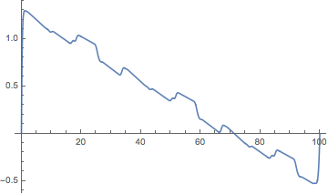
このグラフは、補間とBスプライン関数の変更されたパラメーターの違いを示しています。
Plot[swayTimeCoordinate[t] - t, {t, 0, 100}]
swayOfTime[t_] := sway[swayTimeCoordinate[t]/100][[2]] Plot[swayOfTime[t], {t, 0, 10}]

ツールチップと色付きの長方形を使用して、フレーズとその動きとの関係を視覚化します。
phraseGraphics = BlockMap[ Apply[ Function[{currentAnchor, nextAnchor}, With[ {phraseStart = currentAnchor["PickupBeat"], phraseEnd = nextAnchor["PickupBeat"] - currentAnchor["BeatLength"]}, {Switch[currentAnchor["PhraseName"], "O Christmas Tree", Opacity[0.25, Gray], "Your boughs so green in summertime", Opacity[0.25, Darker@Green], _, Black], Tooltip[ Polygon[ {{phraseStart, -10}, {phraseStart, 10}, {phraseEnd, 10}, {phraseEnd, -10}}], Grid[{{currentAnchor["PhraseName"], SpanFromLeft}, {"Phrase Start:", phraseStart}, {"Phrase End:", phraseEnd} }]]}]]], Append[anchorData0, <|"PickupBeat" -> lastBeat + meanBeatLength|>], 2, 1]; Show[swayControlPointPlot, ParametricPlot[sway[t], {t, 0, Last[measureBeats]}, ImageSize -> Full, PlotPoints -> 800, AspectRatio -> 1/8, PlotTheme -> "Detailed", PlotRangePadding -> Scaled[.02]], Prolog -> phraseGraphics]

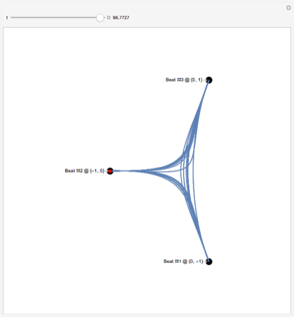
指揮者の動き
指揮者は、音楽と同期した単純な周期的な動きを実行します。
threePatternPoints = {{0, -1}, {-1, -0}, {0, 1}}; threePatternBackground = ListPlot[ MapIndexed[ Callout[#1, StringTemplate["Beat #`` @ ``"][First@#2, #1], Left] &, threePatternPoints], PlotTheme -> "Minimal", Axes -> False, AspectRatio -> 1, PlotStyle -> Directive[Black, PointSize[0.025]], PlotRange -> {{-2, 0.75}, {-1.5, 1.5}}]; conductorControlTimes = swayControlPoints[[All, 1]]; (* basic conductor control points for interpolation *) conductorControlPoints = MapIndexed[{conductorControlTimes[[First[#2]]], #1} &, Join @@ ConstantArray[RotateRight[threePatternPoints, 1], Floor@(Length[conductorControlTimes]/3)]]; (* the shape is okay, but not perfect *) conductor = Interpolation[conductorControlPoints]; (* adding pauses before/after the beat improves the shape of the curves and makes the beats more obvious *) conductorControlPointsWithPauses = Join @@ ({# - {meanBeatLength/8., -0.15* Normalize[ Mean[threePatternPoints] - #[[ 2]]]}, #, # + {meanBeatLength/8., 0.15*Normalize[ Mean[threePatternPoints] - #[[ 2]]]}} & /@ conductorControlPoints);
Interpolation.
conductorWithPauses = Interpolation[conductorControlPointsWithPauses, InterpolationOrder -> 5];
.
Manipulate[ Show[threePatternBackground, ParametricPlot[ conductorWithPauses[t], {t, Max[firstBeat,(*tmax-2*meanBeatLength*)0], tmax}, PerformanceGoal -> "Quality"], Epilog -> {Red, PointSize[Large], Point[conductorWithPauses[tmax]]}, ImageSize -> Large], {{tmax, lastBeat, "t"}, firstBeat + 0.0001, lastBeat, Appearance -> "Labeled"}, SaveDefinitions -> True]
. : , — .
1
2D : : :
δDelay = 0.3; voiceστ[j_][time_] := If[0 < time < tMax,(* smoothing factor *) Sin[Pi time/tMax]^0.25 {voiceFunction[j][1. time] - voiceFunction[j][time - δDelay], voiceFunction[j][1. time]}, {0, 0}] ParametricPlot[voiceστ[1][t], {t, 0, tMax}, AspectRatio -> 1, PlotRange -> All, Frame -> True, Axes -> False, PlotStyle -> Thickness[0.002]]
2
2D : : :
value = -1; interpolateDance[{{t1_, t2_}, {t3_, t4_}}, t_] := With[{y1 = value, y2 = value = -value}, {{y1, t1 < t < t2}, {((y1 - y2) t - (t3 y1 - t2 y2))/(t2 - t3), t2 < t < t3}}]; dancingPositionPiecewise[notes : {__SoundNote}] := With[{noteTimes = Cases[notes, SoundNote[_, times : {startTime_, endTime_}, ___] :> times]}, value = -1; Quiet[Piecewise[ DeleteDuplicatesBy[ Join @@ BlockMap[interpolateDance[#, t] &, noteTimes, 2, 1], Last], 0] ]]; tEnd = Max[voices[[All, All, 2]]]; dancingPositions = dancingPositionPiecewise /@ voices; Plot[Evaluate[KeyValueMap[Legended[#2, #1] &, dancingPositions]], {t, 0, 50}, PlotRangePadding -> Scaled[.05], PlotRange -> {All, {-1, 1}}, ImageSize -> Large, PlotTheme -> "Detailed", PlotLegends -> None]

dancingPositionPiecewiseList = Normal[dancingPositions][[All, 2]]; bsp = BSplineFunction[ Table[Evaluate[{t, dancingPositionPiecewiseList[[2]]}], {t, 0, 100, 0.2}]]
ParametricPlot[bsp[t], {t, 0, 1}, AspectRatio -> 1/4, PlotPoints -> 2000]

Do[voiceIF[j] = BSplineFunction[ Table[Evaluate[{t, dancingPositionPiecewiseList[[j]]}], {t, 0, 100, 0.2}]], {j, 4}] Do[With[{j = j}, voiceTimeCoordinate[j] = Interpolation[Table[{t, voiceIF[j][t/100][[1]]}, {t, 0, 100, 0.1}], InterpolationOrder -> 1]], {j, 4}]
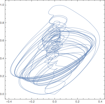
σ-τ [-1,1] * [- 1,1].
Clear[voiceστ]; voiceστ[j_][time_] := If[0 < time < tMax,(* smoothing factor *) Sin[Pi time/tMax]^0.25* {sway[swayTimeCoordinate[time]/tMax][[2]], voiceIF[j][voiceTimeCoordinate[j][time]/tMax][[2]]}, {0, 0}] Table[ListPlot[Table[ voiceστ[j][t], {t, 0, 105, 0.01}], Joined -> True, AspectRatio -> 1, PlotStyle -> Thickness[0.002]], {j, 4}]

() . (, ) . , , , voiceστ [j] [time].
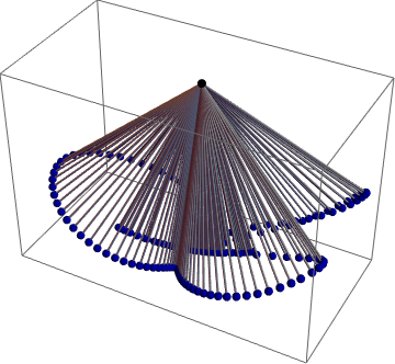
.
Clear[r, ρ, R, X, Y, Z] R[t_] := {X[t], Y[t], Z[t]} r[t_] := R[t] + L {Cos[ϕ[t]] Sin[θ[t]], Sin[ϕ[t]] Sin[θ[t]], -Cos[θ[t]]} ℒ = 1/2 r'[t].r'[t] - gr[t][[3]]
-g (-L Cos[θ[t]] + Z[t]) + 1/2 ((Derivative[1][Z][t] + L Sin[θ[t]] Derivative[1][θ][t])^2 + (Derivative[ 1][Y][t] + L Cos[θ[t]] Sin[ϕ[t]] Derivative[1][θ][t] + L Cos[ϕ[t]] Sin[θ[t]] Derivative[1][ϕ][ t])^2 + (Derivative[1][X][t] + L Cos[θ[t]] Cos[ϕ[t]] Derivative[1][θ][t] — L Sin[θ[t]] Sin[ϕ[t]] Derivative[1][ϕ][t])^2)
ℱ .
ℱ = 1/2 (\[ScriptF]ϕ ϕ'[t]^2 + \[ScriptF]θ θ'[t]^2); eoms = {D[D[ℒ, ϕ'[t]], t] - D[ℒ, ϕ[t]] == -D[ℱ, ϕ'[t]], D[D[ℒ, θ'[t]], t] - D[ℒ, θ[t]] == -D[ℱ, θ'[ t]]} // Simplify
{([ScriptF]ϕ + L^2 Sin[2 θ[t]] Derivative[1][θ][t]) Derivative[ 1][ϕ][t] + L Sin[θ[t]] (-Sinϕ[t]t] + Cos[ϕ[t][t] + L Sinθ[t][t]) == 0, [ScriptF]θ Derivative[1][θ][t] + L (g Sin[θ[t]] — L Cos[θ[t]] Sin[θ[t]] Derivative[1][ϕ][t]^2 + Cos[θ[t]] Cosϕ[t]t] + Cos[θ[t]] Sin[ϕ[t]t] + Sin[θ[t][t] + L (θ^′′)[t]) == 0}
, , [ScriptF] φ, [ScriptF] θ.
paramRules = { g -> 10, L -> 1, \[ScriptF]ϕ -> 1, \[ScriptF]θ -> 1}; In[126]:= X[t_] := If[2 Pi < t < 4 Pi, 8 Cos[t], 8]; Y[t_] := If[2 Pi < t < 4 Pi, 4 Sin[t], 0]; Z[t_] := 0; nds = NDSolve[{eoms /. paramRules, ϕ[0] == 1, ϕ'[0] == 0, θ[0] == 0.001, θ'[0] == 0}, {ϕ, θ}, {t, 0, 20}, PrecisionGoal -> 3, AccuracyGoal -> 3]

Plot[Evaluate[{\[Phi][t], \[Theta][t]} /. nds[[1]]], {t, 0, nds[[1, 2, 2, 1, 1, 2]]}, PlotRange -> All]

Graphics3D[ Table[With[{P = r[t] - R[t] /. nds[[1]] /. paramRules}, {Black, Sphere[{0, 0, 0}, 0.02], Gray, Cylinder[{{0, 0, 0}, P}, 0.005], Darker[Blue], Sphere[P, 0.02]}], {t, 0, 20, 0.05}], PlotRange -> All]
δ τ , .
branchToVoice = Association[ Flatten[Function[{v, bs}, (# -> v) & /@ bs] @@@ Normal[voiceBranches]]]
<|2 -> 1, 9 -> 1, 14 -> 1, 17 -> 1, 19 -> 1, 24 -> 1, 27 -> 1, 3 -> 2, 13 -> 2, 15 -> 2, 16 -> 2, 21 -> 2, 26 -> 2, 1 -> 3, 4 -> 3, 5 -> 3,
12 -> 3, 18 -> 3, 20 -> 3, 6 -> 4, 8 -> 4, 10 -> 4, 11 -> 4, 22 -> 4, 23 -> 4, 25 -> 4|>
tValues = Table[1. t , {t, -5, 110, 0.1}]; Do[στValues = Table[voiceστ[j][t] , {t, -5, 110, 0.1}]; ifσ[j] = Interpolation[ Transpose[{tValues, στValues[[All, 1]]}]]; ifτ[j] = Interpolation[ Transpose[{tValues, στValues[[All, 2]]}]], {j, 4}]
, . , ( ).
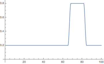
( ) .
changeTimeList = {17.6, 42.2, 66.8, 83.1}; loudness[t_] := With[{λ1 = 0.2, λ2 = 0.8, δt = 1.5}, Which[t <= changeTimeList[[3]] - δt, λ1, changeTimeList[[3]] - δt <= t <= changeTimeList[[3]] + δt, λ1 + (λ2 - 1 λ1) (1 - Cos[Pi (t - (changeTimeList[[ 3]] - δt))/(2 δt)])/2, changeTimeList[[3]] + δt <= t <= changeTimeList[[4]] - δt , λ2, changeTimeList[[4]] - δt <= t <= changeTimeList[[4]] + δt, λ1 + (λ2 - 1 λ1) (1 + Cos[Pi (t - (changeTimeList[[ 4]] - δt))/(2 δt)])/2, t >= changeTimeList[[3]] + 1.5, λ1] ] Plot[loudness[t], {t, 1, 100}, AxesOrigin -> {0, 0}, PlotRange -> All]
Off[General::stop]; SeedRandom[111]; Monitor[ Do[ branchEnd[j, {σ_, τ_}] = branchOnStemEndPoint[ allBranches[[j]], {τ, σ}]; If[j =!= conductorBranch, With[{v = branchToVoice[j]}, tipPosition[t_] = branchEnd[j, loudness[t] {ifσ[v][t], ifτ[v][t]}]]; {X[t_], Y[t_], Z[t_] } = tipPosition[t]; paramRules = { g -> 20, L -> 1, \[ScriptF]ϕ -> 1, \[ScriptF]θ -> 1}; While[ Check[ pendulumϕθ[j][t_] = NDSolveValue[{eoms /. paramRules, ϕ[0] == RandomReal[{-Pi, Pi}], ϕ'[0] == 0.01 RandomReal[{-1, 1}], θ[0] == 0.01 RandomReal[{-1, 1}], θ'[0] == 0.01 RandomReal[{-1, 1}]}, {ϕ[t], θ[t]}, {t, 0, 105}, PrecisionGoal -> 4, AccuracyGoal -> 4, MaxStepSize -> 0.01, MaxSteps -> 100000, Method -> "BDF"]; False, True]] // Quiet], {j, Length[allBranches]}], j]
. .
Plot[pendulum\[Phi]\[Theta][51][t][[2]], {t, 0, 105}, AspectRatio -> 1/4, PlotRange -> All]

.
SeedRandom[11]; Do[randomColor[j] = RandomColor[]; randomAngle[j] = RandomReal[{-Pi/2, Pi/2}], {j, Length[allBranches]}]
.
conductorστ[t_] := Piecewise[ {{{0, 0}, t <= firstBeat/ 2}, {(t - firstBeat/2)/(firstBeat/2) conductorControlPointsWithPauses[[ 1, 2]], firstBeat/2 < t <= firstBeat}, {conductorWithPauses[t], firstBeat < t <= lastBeat}, {(tMax - t)/(tMax - lastBeat) conductorControlPointsWithPauses[[-1, 2]], lastBeat < t < tMax}, {{0, 0}, t >= tMax}}]
.
ListPlot[{Table[{t, conductorστ[t][[1]]}, {t, -1, 3, 0.01}], Table[{t, conductorστ[t][[2]]}, {t, -1, 3, 0.01}]}, PlotRange -> All, Joined -> True]

With[{animationType = 2}, scalefactors[1][t_] := Switch[animationType, 1, {0.8, 1} , 2, loudness[t]]; scalefactors[2][t_] := Switch[animationType, 1, {1, 1} , 2, loudness[t]]; scalefactors[3][t_] := Switch[animationType, 1, {1, 1} , 2, loudness[t]]; scalefactors[4][t_] := Switch[animationType, 1, {1, 1} , 2, loudness[t]] ] christmasTreeWithSwingingOrnaments[t_, conductorEnhancementFactor : fc_, conductorCandleAngle : ωc_, topRotationAngle : ω_, opts___] := Graphics3D[{{Darker[Brown], stem}, (* first voice *) branchOnStemWithBall[allBranches[[#]], scalefactors[1][t] voiceστ[1][t], Darker[Yellow, -0.1], If[t < 0, {0, 0}, pendulumϕθ[#][t]]] & /@ voiceBranches[[1]], (* second voice *) branchOnStemWithBall[allBranches[[#]], scalefactors[2] [t] voiceστ[2][t], Blend[{Red, Pink}], If[t < 0, {0, 0}, pendulumϕθ[#][t]]] & /@ voiceBranches[[2]], (* third voice *) branchOnStemWithFiveStar[allBranches[[#]], scalefactors[3][t] voiceστ[3][t], randomColor[#], Pi/4, If[t < 0, {0, 0}, pendulumϕθ[#][t]]] & /@ voiceBranches[[3]], (* fourth voice *) branchOnStemWithCandle[#, scalefactors[4][t] voiceστ[4][t], Directive[White, Glow[GrayLevel[0.3]], Specularity[Yellow, 20]], 0] & /@ allBranches[[voiceBranches[[4]]]], (* conductor *) branchOnStemWithCandle[ allBranches[[conductorBranch]] {1, 1, 1 + fc}, conductorστ[t], Directive[Red, Glow[GrayLevel[0.1]], Specularity[Yellow, 20]], ωc], Rotate[top, ω, {0, 0, 1}] }, opts, ViewPoint -> {2.8, 1.79, 0.1}, PlotRange -> {{-8, 8}, {-8, 8}, {-2, 15}}, Background -> RGBColor[0.998, 1., 0.867] ]
, .
Show[christmasTreeWithSwingingOrnaments[70, 0.5, 0.8, 2], PlotRange -> All, Boxed -> False]

!
() . , 3D-, . , PDE (http://psoup.math.wisc.edu/papers/h3l.pdf), , , .
(2D)
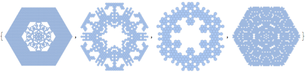
- « - ». , hex snowflake.
ReleaseHold /@ (MakeExpression[#[[1]], StandardForm] & /@ Take[Cases[ Import["http://demonstrations.wolfram.com/downloadauthornb.cgi?\ name=SnowflakeLikePatterns"], Cell[_, "Input", ___], ∞], 2]); makeSnowflake[rule_, steps_] := Polygon[hex[#] & /@ Select[Position[Reverse[CellularAutomaton[ {snowflakes[[ rule]], {2, {{0, 2, 2}, {2, 1, 2}, {2, 2, 0}}}, {1, 1}}, {{{1}}, 0}, {{{steps}}, {-steps, steps}, {-steps, steps}}]], 0], -steps - 1 < -#[[1]] + #[[2]] < steps + 1 &]] SeedRandom[33]; Table[Graphics[{Darker[Blue], makeSnowflake[RandomInteger[{1, 3888}], RandomInteger[{10, 60}]]}], {4}]

, , . , .
denseFlakeQ[mr_MeshRegion] := With[{c = RegionCentroid[mr], pts = MeshCoordinates[mr]}, ( Divide @@ MinMax[EuclideanDistance[c, #] & /@ pts]) < 1/3] randomSnowflakes[] := Module[{sf}, While[(sf = Module[{}, TimeConstrained[ hexagons = makeSnowflake[RandomInteger[{1, 3888}], RandomInteger[{10, 60}]]; (Select[ConnectedMeshComponents[DiscretizeRegion[hexagons]], (Area[#] > 120 && Perimeter[#]/Area[#] < 2 && denseFlakeQ[#]) &] /. \ _ConnectedMeshComponents :> {}) // Quiet, 20, {}]]) === {}]; sf] randomSnowflakes[n_] := Take[NestWhile[Join[#, randomSnowflakes[]] &, {}, Length[#] < n &], n] SeedRandom[22]; randomSnowflakes[4]
normalizeFlake[mr_MeshRegion] := Module[{coords, center, coords1, size, coords2}, coords = MeshCoordinates[mr]; center = Mean[coords]; coords1 = (# - center) & /@ coords; size = Max[Norm /@ coords1]; coords2 = coords1/size; GraphicsComplex[coords2, {EdgeForm[], MeshCells[mr, 2]}]]
.

(3D)
2D , , 3D .
make3DFlake[flake2D_] := Module[{grc, reg, boundary, h, bc, rb, polys, pts}, grc = flake2D[[1]]; reg = MeshRegion @@ (grc /. _EdgeForm :> Nothing); boundary = (MeshPrimitives[#, 1] &@RegionBoundary[reg])[[All, 1]]; h = RandomReal[{0.05, 0.15}]; bc = Join[#1, Reverse[#2]] & @@@ Transpose[{Map[Append[#, 0] &, boundary, {-2}], Map[Append[#, h] &, boundary, {-2}]}]; rb = RegionBoundary[reg]; boundary = (MeshCells[#, 1] &@rb)[[All, 1]]; polys = Polygon[Join[#1, Reverse[#2]] & @@@ Transpose[{boundary, boundary + Max[boundary]}]]; pts = Join[Append[#, 0] & /@ MeshCoordinates[rb], Append[#, h] & /@ MeshCoordinates[rb]]; {GraphicsComplex[Developer`ToPackedArray[pts], polys], MapAt[Developer`ToPackedArray[Append[#, 0]] & /@ # &, flake2D[[1]], 1], MapAt[Developer`ToPackedArray[Append[#, h]] & /@ # &, flake2D[[1]], 1]} ] listOfSnowflakes3D = make3DFlake /@ listOfSnowflakes; Graphics3D[{EdgeForm[], #}, Boxed -> False, Method -> {"ShrinkWrap" -> True}, ImageSize -> 120, Lighting -> {{"Ambient", Hue[.58, .5, 1]}, {"Directional", GrayLevel[.3], ImageScaled[{1, 1, 0}]}}] & /@ listOfSnowflakes3D

1994 . , , .
Manipulate[ Module[{eqs, nds, tmax, g = 10, α, sign, V, x, y, u, v, θ, ω, kpar = kperp/f, ρ = 10^ρexp}, α = ArcTan[u[t], v[t]]; sign = Piecewise[{{1, (v[t] < 0 && 0 <= α + θ[t] <= Pi) || (v[t] > 0 && -Pi <= α + θ[t] <= 0)}}, -1]; V = Sqrt[u[t]^2 + v[t]^2]; eqs = {D[x[t], t] == u[t], D[y[t], t] == v[t], D[u[t], t] == -(kperp Sin[θ[t]]^2 + kpar Cos[θ[t]]^2) u[ t] + (kperp - kpar) Sin[θ[ t]] Cos[θ[t]] v[t] - sign Pi ρ V^2 Cos[α + θ[t]] Cos[α], D[v[t], t] == -(kperp Cos[θ[t]]^2 + kpar Sin[θ[t]]^2) v[ t] + (kperp - kpar) Sin[θ[ t]] Cos[θ[t]] u[t] + sign Pi ρ V^2 Cos[α + θ[ t]] Sin[α] - g, D[ω[t], t] == -kperp ω[ t] - (3 Pi ρ V^2/l) Cos[α + θ[ t]] Sin[α + θ[t]], D[θ[t], t] == ω[t]} /. kpar -> kperp/f; nds = NDSolve[ Join[eqs, {x[0] == 0, y[0] == 0, u[0] == 0, v[0] == 0.01, ω[0] == 0, θ[0] == θ0}], {x, y, u, v, θ, ω}, {t, 0, T}, MaxSteps -> 2000] // Quiet; tmax = nds[[1, 2, 2, 1, 1, 2]]; Graphics[{Thickness[0.002], Gray, Table[Evaluate[ Line[{{x[t], y[t]} - l/2 {Cos[θ[t]], Sin[θ[t]]}, {x[t], y[t]} + l/2 {Cos[θ[t]], Sin[θ[t]]}}] /. nds[[1]]], {t, 0, tmax, tmax/n}], Blue, Line[Table[ Evaluate[{x[t], y[t]} /. nds[[1]]], {t, 0, tmax, tmax/200}]]}, AspectRatio -> ar, Frame -> True, PlotRange -> All]], "system parameters", {{kperp, 5.1, Subscript["k", "∟"]}, 0.01, 10, Appearance -> "Labeled"}, {{f, 145, Row[{Subscript["k", "∟"], "/", Subscript["k", "∥"]}]}, 0.01, 200, Appearance -> "Labeled"}, {{ρexp, -0.45, Log["ρ"]}, -3, 1, Appearance -> "Labeled"}, {{l, 0.63}, 0.01, 10, Appearance -> "Labeled"} , Delimiter, "fall parameters", {{θ0, 1, Subscript["θ", "0"]}, -Pi, Pi, Appearance -> "Labeled"}, {{T, 2, "falling time"}, 0, 10, Appearance -> "Labeled"} , Delimiter, "plot", {{ar, 1, "aspect ratio"}, {1, Automatic}}, {{n, 200, "snapshots"}, 2, 500, 1}]

, . / , .
, .
randomParametrizedRotationMatrix[n_, τ_] := Function @@ {τ, Module[{phi, s, c}, Do[phi[i] = Sum[RandomReal[{-1, 1}] Sin[ RandomReal[{0, n}] τ + 2 Pi RandomReal[]], {n}]; {c[i], s[i]} = {Cos[phi[i]], Sin[phi[i]]}, {i, 3}]; {{c[1], s[1], 0}, {-s[1], c[1], 0}, {0, 0, 1}}. {{c[2], 0, s[2]}, {0, 1, 0}, {-s[2], 0, c[2]}}. {{1, 0, 0}, {0, c[3], s[3]}, {0, -s[3], c[3]}}]}; randomParametrizedPathFunction := Function[t, Evaluate[{RandomReal[{-5, 5}] + Sum[RandomReal[{-1, 1}]/# Cos[2 Pi # t] &[ RandomReal[{1, 4}]], {k, 5}], RandomReal[{-5, 5}] + Sum[RandomReal[{-1, 1}]/# Cos[2 Pi # t] &[ RandomReal[{1, 4}]], {k, 5}], RandomReal[{2, 12}] - RandomReal[{1.5, 2.5}] t}]] SeedRandom[55]; Do[rotMat[j] = randomParametrizedRotationMatrix[3, τ]; trans[j] = randomParametrizedPathFunction; snowflakeColor[ j] = {{"Ambient", Hue[RandomReal[{0.55, 0.6}], RandomReal[{0.48, 0.52}], RandomReal[{0.95, 1}]]}, {"Directional", GrayLevel[RandomReal[{0.28, 0.32}]], ImageScaled[{1, 1, 0}]}}, {j, Length[listOfSnowflakes]}] fallingSnowflake[flake_, {t_, ℛ_}] := flake /. GraphicsComplex[cs_, rest__] :> GraphicsComplex[(ℛ.# + t) & /@ cs, rest] Manipulate[ Graphics3D[{EdgeForm[], Table[{Lighting -> snowflakeColor[k], fallingSnowflake[ listOfSnowflakes3D[[k]], {trans[k][t], rotMat[k][t]}]}, {k, Length[listOfSnowflakes3D]}] }, PlotRange -> 6, ViewPoint -> {0, -10, 0}, ImageSize -> 400], {{t, 3.2}, -5, 20}]

.
, , . . , . , , . 24 .
conductorBranchMaxfactor = 0.5; conductorBranchLength[t_] := conductorBranchMaxfactor* Which[t < -3, 0, -3 < t <= 0, (t + 3)/3., 0 <= t <= tMax, 1, tMax < t < tMax + 3, (1 - (t - tMax)/3), True, 0]; topRotation[t_] := Which[t < -3 || t > tMax + 3, 0, True, (1. - Cos[(t + 3)/(tMax + 6)]) 20 2 Pi]; viewPoint[t_] := With[{vp = {2.8, 1.79, 0.1}}, Which[t < changeTimeList[[1]] || t > changeTimeList[[2]], vp, changeTimeList[[1]] <= t <= changeTimeList[[2]], Module[{t0 = changeTimeList[[1]], Δt = changeTimeList[[2]] - changeTimeList[[1]], ωvp}, ωvp = -Pi (1 - Cos[ Pi (t - t0)/Δt]); {{Cos[ωvp], Sin[ωvp], 0}, {-Sin[ωvp], Cos[ωvp], 0}, {0, 0, 1}}.vp + {0, 0, 2 Sin[Pi (t - t0)/Δt]^4 }]]] ParametricPlot3D[ viewPoint[t], {t, changeTimeList[[1]], changeTimeList[[2]]}, BoxRatios -> {1, 1, 1}]

animationFrame[t_] := Show[christmasTreeWithSwingingOrnaments[t, conductorBranchLength[t], 1.4 conductorBranchLength[t], topRotation[t]], Background -> None, Boxed -> False, SphericalRegion -> True, ViewPoint -> viewPoint[t]]
, :
animationFrame[35]

framesPerSecond = 24; animationFrameDirectory = "/Users/mtrott/Desktop/ConductingChristmasTreeAnimationFrames/"; Monitor[ Do[ With[{t = -3 + 1/framesPerSecond (frame - 1)}, gr = animationFrame[t]; Export[animationFrameDirectory <> IntegerString[frame, 10, 4] <> ".png", gr, ImageSize -> 1800, Background -> None] ], {frame, 1, framesPerSecond (100 + 2 3)}], Row[{frame, " | ", Round[MemoryInUse[]/1024^2], "\[ThinSpace]MB" }] ]
(, Adobe After Effects) , .
info-russia@wolfram.com
Mathematica
Wolfram|One