ここにいくつかの変更を加えた記事のコードを示します。特に、「順列」ブロックに注意を払うようにお願いします。好奇心を紹介し、満足させます。
from keras.datasets import mnist from keras.models import Model from keras.layers import Input, Dense from keras.utils import np_utils import numpy as np %matplotlib inline import matplotlib.pyplot as plt batch_size = 128 num_epochs = 16 hidden_size_1 = 512 hidden_size_2 = 512 height, width, depth = 28, 28, 1 # MNIST images are 28x28 and greyscale num_classes = 10 # there are 10 classes (1 per digit) (X_train, y_train), (X_test, y_test) = mnist.load_data() # fetch MNIST data num_train, width, depth = X_train.shape num_test = X_test.shape[0] num_classes = np.unique(y_train).shape[0] # there are 10 image classes #Visualizing I_train = list() I_test = list() fig, axes = plt.subplots(1,10,figsize=(10,10)) for k in range(10): i = np.random.choice(range(len(X_train))) I_train.append(i) axes[k].set_axis_off() axes[k].imshow(X_train[i:i+1][0], cmap='gray') fig, axes = plt.subplots(1,10,figsize=(10,10)) for k in range(10): i = np.random.choice(range(len(X_test))) I_test.append(i) axes[k].set_axis_off() axes[k].imshow(X_test[i:i+1][0], cmap='gray') X_train = X_train.reshape(num_train, height * width) X_test = X_test.reshape(num_test, height * width) XX_test = np.copy(X_test) XX_train = np.copy(X_train)
元の写真を読む(どのような写真とその理由-元の記事を読んでください)
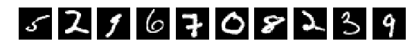
そして、Train and Testから10個をランダムに選択して表示しました。 絵としての絵、何も変更されていない場合(perm = np.arange(28 * 28))、ネットワークは98%以上を与えます。 わかった
自分で確認できます。
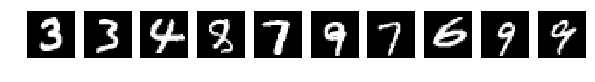
しかし、今では写真をランダムにミックスします。 偶然ですが、偶然ですが、すべての画像が同じように干渉します。
# perm = np.random.permutation((28*28)) # for j in xrange(X_test.shape[1]): for i in xrange(X_test.shape[0]): X_test[i][j] = XX_test[i][perm[j]] for i in xrange(X_train.shape[0]): X_train[i][j] = XX_train[i][perm[j]] #
写真を見て、ネットワークを開始します。
X_train = X_train.reshape(num_train, height, width) X_test = X_test.reshape(num_test, height, width) #Visualizing fig, axes = plt.subplots(1,10,figsize=(10,10)) for k in range(10): i = I_train[k] axes[k].set_axis_off() axes[k].imshow(X_train[i:i+1][0], cmap='gray') fig, axes = plt.subplots(1,10,figsize=(10,10)) for k in range(10): i = I_test[k] axes[k].set_axis_off() axes[k].imshow(X_test[i:i+1][0], cmap='gray') X_train = X_train.reshape(num_train, height * width) # Flatten data to 1D X_test = X_test.reshape(num_test, height * width) # Flatten data to 1D X_train = X_train.astype('float32') X_test = X_test.astype('float32') X_train /= np.max(X_train) # Normalise data to [0, 1] range X_test /= np.max(X_test) # Normalise data to [0, 1] range Y_train = np_utils.to_categorical(y_train, num_classes) # One-hot encode the labels Y_test = np_utils.to_categorical(y_test, num_classes) # One-hot encode the labels inp = Input(shape=(height * width,)) # Our input is a 1D vector of size 784 hidden_1 = Dense(hidden_size_1, activation='relu')(inp) # First hidden ReLU layer hidden_2 = Dense(hidden_size_2, activation='relu')(hidden_1) # Second hidden ReLU layer out = Dense(num_classes, activation='softmax')(hidden_2) # Output softmax layer model = Model(input=inp, output=out) # To define a model, just specify its input and output layers model.compile(loss='categorical_crossentropy', # using the cross-entropy loss function optimizer='adam', # using the Adam optimiser metrics=['accuracy']) # reporting the accuracy model.fit(X_train, Y_train, # Train the model using the training set... batch_size=batch_size, nb_epoch=num_epochs, verbose=1, validation_split=0.1) # ...holding out 10% of the data for validation model.evaluate(X_test, Y_test, verbose=1) # Evaluate the trained model on the test set!
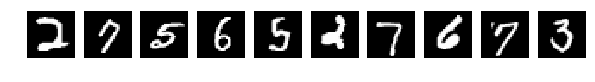
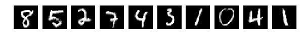
元のランダムに選択された10枚の写真を、今では同じものを混合した後。
すべての写真が同じ方法で混合されたことを思い出させてください。
しかし、ここでああ! 神秘主義、ネットワークはそのような写真に簡単に対処でき、[0.082131341451834983、0.98219999999999996]を取得します。
このような混合写真では、誰もそのようなタスクに対処できません。 これは輝いている!!! これは人間と比較して驚異的です。 何千年もの間、北斗七星と弓を探してください。
しかし、探究心はそこに止まらず、今、揺れようとしている。 より正確には、別のコードを適用します。
for j in xrange(X_test.shape[1]): for i in xrange(X_test.shape[0]): X_test[i][j] = perm[XX_test[i][j]] for i in xrange(X_train.shape[0]): X_train[i][j] = perm[XX_train[i][j]]
ポイントが混在しているのではなく、ポイントの値が混在しています。 再びランダムにミックスできますが、主なものは写真全体で同じですが、ミキシングで非常に広く知られているものを選択できます。
perm = np.array([ 0x63, 0x7c, 0x77, 0x7b, 0xf2, 0x6b, 0x6f, 0xc5, 0x30, 0x01, 0x67, 0x2b, 0xfe, 0xd7, 0xab, 0x76, 0xca, 0x82, 0xc9, 0x7d, 0xfa, 0x59, 0x47, 0xf0, 0xad, 0xd4, 0xa2, 0xaf, 0x9c, 0xa4, 0x72, 0xc0, 0xb7, 0xfd, 0x93, 0x26, 0x36, 0x3f, 0xf7, 0xcc, 0x34, 0xa5, 0xe5, 0xf1, 0x71, 0xd8, 0x31, 0x15, 0x04, 0xc7, 0x23, 0xc3, 0x18, 0x96, 0x05, 0x9a, 0x07, 0x12, 0x80, 0xe2, 0xeb, 0x27, 0xb2, 0x75, 0x09, 0x83, 0x2c, 0x1a, 0x1b, 0x6e, 0x5a, 0xa0, 0x52, 0x3b, 0xd6, 0xb3, 0x29, 0xe3, 0x2f, 0x84, 0x53, 0xd1, 0x00, 0xed, 0x20, 0xfc, 0xb1, 0x5b, 0x6a, 0xcb, 0xbe, 0x39, 0x4a, 0x4c, 0x58, 0xcf, 0xd0, 0xef, 0xaa, 0xfb, 0x43, 0x4d, 0x33, 0x85, 0x45, 0xf9, 0x02, 0x7f, 0x50, 0x3c, 0x9f, 0xa8, 0x51, 0xa3, 0x40, 0x8f, 0x92, 0x9d, 0x38, 0xf5, 0xbc, 0xb6, 0xda, 0x21, 0x10, 0xff, 0xf3, 0xd2, 0xcd, 0x0c, 0x13, 0xec, 0x5f, 0x97, 0x44, 0x17, 0xc4, 0xa7, 0x7e, 0x3d, 0x64, 0x5d, 0x19, 0x73, 0x60, 0x81, 0x4f, 0xdc, 0x22, 0x2a, 0x90, 0x88, 0x46, 0xee, 0xb8, 0x14, 0xde, 0x5e, 0x0b, 0xdb, 0xe0, 0x32, 0x3a, 0x0a, 0x49, 0x06, 0x24, 0x5c, 0xc2, 0xd3, 0xac, 0x62, 0x91, 0x95, 0xe4, 0x79, 0xe7, 0xc8, 0x37, 0x6d, 0x8d, 0xd5, 0x4e, 0xa9, 0x6c, 0x56, 0xf4, 0xea, 0x65, 0x7a, 0xae, 0x08, 0xba, 0x78, 0x25, 0x2e, 0x1c, 0xa6, 0xb4, 0xc6, 0xe8, 0xdd, 0x74, 0x1f, 0x4b, 0xbd, 0x8b, 0x8a, 0x70, 0x3e, 0xb5, 0x66, 0x48, 0x03, 0xf6, 0x0e, 0x61, 0x35, 0x57, 0xb9, 0x86, 0xc1, 0x1d, 0x9e, 0xe1, 0xf8, 0x98, 0x11, 0x69, 0xd9, 0x8e, 0x94, 0x9b, 0x1e, 0x87, 0xe9, 0xce, 0x55, 0x28, 0xdf, 0x8c, 0xa1, 0x89, 0x0d, 0xbf, 0xe6, 0x42, 0x68, 0x41, 0x99, 0x2d, 0x0f, 0xb0, 0x54, 0xbb, 0x16])
そして、ネットワークの結果(変更なしの同じコード)がすぐに警告されました:
[1.0329392189979554、0.64970000000000006]


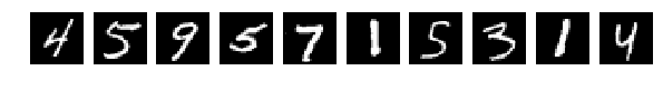
目で見ると、どの数字がどこにあるかを明確に理解できますが、ネットワークの結果は憂鬱です。 振ると結果が著しく悪化しました。
そして最後に、軟膏のハエ。
もし
perm = np.array([ 153, 17, 7, 148, 191, 15, 73, 109, 180, 129, 2, 218, 122, 151, 227, 167, 40, 248, 66, 212, 197, 101, 211, 139, 234, 133, 168, 174, 53, 207, 219, 37, 246, 194, 239, 255, 107, 90, 22, 44, 215, 84, 102, 201, 61, 176, 72, 125, 56, 99, 156, 161, 226, 6, 238, 52, 27, 50, 216, 231, 71, 5, 25, 34, 62, 29, 166, 253, 220, 3, 24, 225, 130, 196, 113, 86, 150, 209, 65, 195, 1, 200, 41, 81, 69, 163, 33, 147, 230, 202, 232, 112, 241, 137, 47, 187, 203, 175, 229, 39, 160, 186, 152, 222, 14, 85, 21, 77, 210, 108, 193, 250, 54, 45, 92, 141, 94, 208, 110, 192, 228, 115, 91, 143, 26, 88, 96, 170, 78, 87, 132, 172, 247, 178, 205, 165, 177, 144, 83, 49, 11, 67, 82, 134, 245, 100, 18, 48, 136, 213, 105, 162, 199, 103, 252, 214, 158, 189, 149, 95, 164, 111, 233, 181, 142, 249, 9, 236, 38, 173, 243, 57, 28, 128, 55, 32, 116, 59, 145, 97, 35, 106, 43, 206, 198, 60, 135, 74, 23, 76, 251, 120, 240, 75, 20, 169, 179, 121, 80, 217, 123, 235, 126, 114, 16, 155, 146, 119, 19, 8, 51, 98, 42, 185, 127, 93, 190, 104, 224, 171, 244, 124, 89, 68, 0, 4, 117, 182, 70, 64, 159, 157, 242, 188, 10, 30, 36, 58, 138, 118, 204, 184, 221, 13, 254, 31, 12, 140, 63, 223, 79, 46, 154, 183, 131, 237])
その後、すべてが完全に悪いです。


すべてが目で見えるが、ネットワークは解放する
[2.301039520263672、0.1135]
結論:「かくはんしますが、振らないでください。」
PS。 記事は不完全感を残します。 書かなければなりませんでした
モンスターとブロンドについて続けた