
The world around us is filled with all kinds of information that our brain continuously processes. He receives this information through the senses, each of which is responsible for its share of signals: eyes (vision), tongue (taste), nose (smell), skin (touch), vestibular apparatus (balance, spatial position and sense of weight) and ears (sound). By putting together signals from all these organs, our brain can build an accurate picture of the environment. But not all aspects of external signal processing are known to us. One of these secrets is the localization mechanism of the sound source.
Scientists from the Neuroengineering Laboratory for Speech and Hearing (New Jersey Institute of Technology) have proposed a new model of the neural process of sound localization. What exactly processes occur in the brain during the perception of sound, how our brain understands the position of the sound source and how this study can help in the fight against hearing defects. We learn about this from the report of the research group. Go.
Study basis
The information that our brain receives from the senses differs from each other both in terms of source and in terms of its processing. Some signals immediately appear in front of our brain in the form of accurate information, while others need additional computational processes. Roughly speaking, we feel the touch right away, but when we hear the sound, we still have to find where it comes from.
The basis for localizing sounds in the horizontal plane is the interaural * time difference (ITD from interaural time difference ) of sounds reaching the listener's ears.
Interaural base * - the distance between the ears.There is a certain area in the brain (medial superior olive or MBO) that is responsible for this process. At the time of receiving the sound signal in the MBO, the interaural differences in time are converted into the reaction rate of neurons. The shape of the velocity curves of the output signal of the MBO as a function of ITD resembles the shape of the cross-correlation function of the input signals for each ear.
The way information is processed and interpreted in the MBO remains not completely clear, which is why there are several very conflicting theories. The most famous and in fact classical theory of sound localization is the Jeffress model ( Lloyd A. Jeffress ). It is based on a marked line * of neuron detectors that are sensitive to binaural synchronism of neural input signals from each ear, and each neuron is most sensitive to a specific ITD value ( 1A ).
The principle of the marked line * is a hypothesis that explains how different nerves, all of which use the same physiological principles to transmit impulses along their axons, are able to generate different sensations. Structurally similar nerves can generate different sensory perceptions if they are associated with unique neurons in the central nervous system that are able to decode similar nerve signals in various ways.

Image No. 1
This model is computationally similar to neural coding based on unlimited cross-correlations of sounds reaching both ears.
There is also a model in which it is assumed that the localization of sound can be modeled on the basis of differences in the reaction rate of certain populations of neurons from different hemispheres of the brain, i.e. model of interhemispheric asymmetry ( 1B ).
Until now, it was difficult to unequivocally state which of the two theories (models) is correct, given that each of them predicts different dependences of sound localization on sound intensity.
In the study we are considering today, scientists decided to combine both models in order to understand whether the perception of sounds is based on neural coding or on the difference in the response of individual neural populations. Several experiments were carried out in which people aged 18 to 27 years (5 women and 7 men) took part. The audiometry (measurement of hearing acuity) of the participants was 25 dB or higher at a frequency of 250 to 8000 Hz. The test participant was placed in a soundproof room in which special equipment was calibrated with high accuracy. Participants should, having heard a sound signal, indicate the direction from which it comes.
Research results
To assess the dependence of lateralization * of brain activity on the intensity of sound in response to marked neurons, we used data on the reaction rate of neurons in the laminar core of the barn owl brain.
Laterality * - asymmetry of the left and right halves of the body.To assess the dependence of the lateralization of brain activity on the reaction rate of certain populations of neurons, we used the activity data of the lower two-brain of the rhesus macaque, after which differences in the speed of neurons from different hemispheres were additionally calculated.
The model of the marked line of neuron detectors suggests that with a decrease in sound intensity, the laterality of the perceived source will converge in average values similar to the ratio of quiet and loud sounds ( 1C ).
The interhemispheric asymmetry model, in turn, suggests that with a decrease in sound intensity to almost threshold, the perceived laterality will shift to the midline ( 1D ).
At a higher overall sound intensity, it is assumed that the lateralization will be invariant in intensity (inserts at 1C and 1D ).
Therefore, an analysis of how sound intensity affects the perceived direction of sound allows you to accurately determine the nature of the processes taking place at that moment - neurons from one common area or neurons from different hemispheres.
Obviously, a person’s ability to distinguish between ITDs may vary with sound intensity. However, scientists say that it is difficult to interpret previous findings relating sensitivity to ITD and the listener's assessment of the direction of the sound source as a function of sound intensity. Some studies say that when the sound intensity reaches the boundary threshold, the perceived laterality of the source decreases. Other studies suggest that there is no effect of intensity on perception at all.
In other words, the scientists “gently” hint that there is not enough information in the literature regarding the relationship between ITD, sound intensity, and determining the direction of its source. There are theories that exist as a kind of axioms generally accepted by the scientific community. Therefore, it was decided to test in detail all theories, models, and possible mechanisms of hearing perception in practice.
The first experiment was carried out using the psychophysical paradigm, which allowed us to study ITD-based lateralization as a function of sound intensity in a group of ten normally hearing participants in the experiment.

Image No. 2
Sound sources were specially tuned to cover most of the frequency range within which people are able to recognize ITD, i.e. 300 to 1200 Hz ( 2A ).
In each of the tests, the listener had to indicate the expected laterality, measured as a function of the level of sensations, in the range of ITD values from 375 to 375 ms. To determine the effect of sound intensity, the nonlinear mixed effect model (NMLE) was used, which included both fixed and random sound intensity.
Graph 2B shows the estimated lateralization with spectrally flat noise at two sound intensities for a representative listener. A graph 2C shows the raw data (circles) and tailored to the NMLE model (lines) of all listeners.
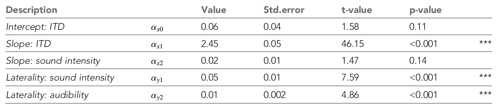
Table number 1
The table above shows all the NLME parameters. It can be seen that perceived laterality increased with an increase in ITD, as scientists had expected. With a decrease in sound intensity, perception shifted more and more towards the midline (insert on the 2C graph).
These trends were reinforced by the NLME model, which showed a significant influence of ITD and sound intensity on the maximum degree of laterality, confirming the model of interhemispheric differences.
In addition, the average audiometric thresholds of pure tones had a negligible effect on perceived laterality. But the sound intensity did not significantly affect the performance of psychometric functions.
The main goal of the second experiment was to determine how the results obtained in the previous experiment will change when the spectral features of stimuli (sounds) are taken into account. The need to test spectrally flat noise at low sound intensities is that parts of the spectrum may not be audible, and this may affect the determination of the direction of sound. Therefore, the fact that the width of the audible part of the spectrum can decrease with decreasing sound intensity can be mistaken for the results of the first experiment.
Therefore, it was decided to conduct another experiment, but already using back A-weighted * noise.
A-weighting * is applied to sound levels to take into account the relative loudness perceived by the human ear, since the ear is less sensitive to low sound frequencies. A-weighting is implemented by arithmetically adding a table of values listed in octave bands to the measured sound pressure levels in dB.The 2D graph shows the raw data (circles) and the data (lines) of the experiment participants tailored to the NMLE model.
An analysis of the data showed that when all parts of the sound are approximately equally audible (both in the first and second experiments), the perceived laterality and slope on the graph explaining the change in laterality with ITD decrease with decreasing sound intensity.
Thus, the results of the second experiment confirmed the results of the first. That is, in practice it was shown that the model proposed back in 1948 by Jeffress is not correct.
It turns out that the localization of sounds worsens with a decrease in sound intensity, and Jeffress believed that sounds are perceived and processed by a person equally regardless of their intensity.
For a more detailed acquaintance with the nuances of the study, I recommend a look at the report of scientists .
Epilogue
Theoretical assumptions and practical experiments confirming them showed that mammalian brain neurons are activated at different speeds depending on the direction of the sound signal. Following this, the brain compares these speeds between all neurons involved in the process to dynamically map the sound environment.
The Jeffresson model is actually not 100% erroneous, since with its help it is possible to perfectly describe the localization of the sound source in a siwuh. Yes, for barn owls, the sound intensity does not matter, they will in any case determine the position of its source. However, this model does not work with rhesus monkeys, as shown by previous experiments. Therefore, this Jeffresson model cannot describe the localization of sounds for all living things.
Experiments with people once again confirmed that the localization of sounds occurs in different organisms in different ways. Many of the participants could not correctly determine the position of the source of sound signals due to the low intensity of the sounds.
Scientists believe that their work shows a certain similarity between the way we see and how we hear. Both processes are associated with the speed of neurons in different parts of the brain, as well as with the assessment of this difference to determine both the position of the objects we see in space and the position of the source of the sound we hear.
In the future, researchers are going to conduct a series of experiments to more closely examine the relationship between human hearing and vision, which will help us better understand how our brain dynamically constructs a map of the world around us.
Thank you for your attention, remain curious and have a good working week, guys! :)
Thank you for staying with us. Do you like our articles? Want to see more interesting materials? Support us by placing an order or recommending it to your friends, cloud VPS for developers from $ 4.99 , a 30% discount for Habr users on the unique entry-level server analog that we invented for you: The whole truth about VPS (KVM) E5-2650 v4 (6 Cores) 10GB DDR4 240GB SSD 1Gbps from $ 20 or how to share a server? (options are available with RAID1 and RAID10, up to 24 cores and up to 40GB DDR4).
Dell R730xd 2 times cheaper? Only we have 2 x Intel TetraDeca-Core Xeon 2x E5-2697v3 2.6GHz 14C 64GB DDR4 4x960GB SSD 1Gbps 100 TV from $ 199 in the Netherlands! Dell R420 - 2x E5-2430 2.2Ghz 6C 128GB DDR3 2x960GB SSD 1Gbps 100TB - from $ 99! Read about How to Build Infrastructure Bldg. class c using Dell R730xd E5-2650 v4 servers costing 9,000 euros for a penny?