From the report of Dmitry Afanasyev, you will learn about the basic principles of the new design, scaling of topologies that arise with these problems, their solutions, about the features of routing and scaling of the forwarding plane functions of modern network devices in “densely connected” topologies with a large number of ECMP routes . In addition, Dima briefly talked about the organization of external connectivity, the physical level, the cable system and ways to further increase capacity.
- Good afternoon, everyone! My name is Dmitry Afanasyev, I am a network architect of Yandex and I mainly deal with the design of data center networks.
My story will be about the updated network of Yandex data centers. This is largely an evolution of the design that we had, but at the same time there are some new elements. This is a review presentation, since it was necessary to fit a lot of information in a short time. We start by choosing a logical topology. Then there will be an overview of the control plane and problems with scalability of the data plane, the choice of what will happen on the physical level, let's look at some features of the devices. We will touch a little and what is happening in the data center with MPLS, about which we spoke some time ago.
So, what is Yandex in terms of workloads and services? Yandex is a typical hyperscaler. If you look at the users, we are primarily processing user requests. Also, various streaming services and data output, because we also have storage services. If closer to the backend, then there are infrastructure loads and services, such as distributed object stores, data replication and, of course, persistent queues. One of the main types of loads is MapReduce and the like, streaming processing, machine learning, etc.
How is the infrastructure on top of which this all happens? Again, we are quite a typical hyperscaler, although perhaps we are a little closer to the side of the spectrum where the smaller hyperscalers are located. But we have all the attributes. We use commodity hardware and horizontal scaling wherever possible. We have a full growth of resource pooling: we do not work with individual machines, separate racks, but combine them into a large pool of interchangeable resources with some additional services that are engaged in planning and allocation, and we work with all of this pool.
So we have the next level - the operating system level computing cluster. It is very important that we fully control the technology stack that we use. We control endpoints (hosts), network and software stack.
We have several large data centers in Russia and abroad. They are united by a backbone using MPLS technology. Our internal infrastructure is almost entirely IPv6-based, but since we need to handle external traffic, which is still mainly delivered via IPv4, we need to somehow deliver requests arriving via IPv4 to the front-end servers, and still go a little to external IPv4- Internet - for example, for indexing.
The last few iterations of data center network design use multi-level Clos topologies, and only L3 is used in them. We left L2 some time ago and breathed a sigh of relief. Finally, our infrastructure includes hundreds of thousands of computing (server) instances. The maximum cluster size some time ago was about 10 thousand servers. This is largely due to how the same cluster-level operating systems — schedulers, resource allocation, etc., can work. Since progress has occurred on the side of infrastructure software, now the target is about 100 thousand servers in one computing cluster, and we had a task - to be able to build network factories that allow efficient pooling of resources in such a cluster.
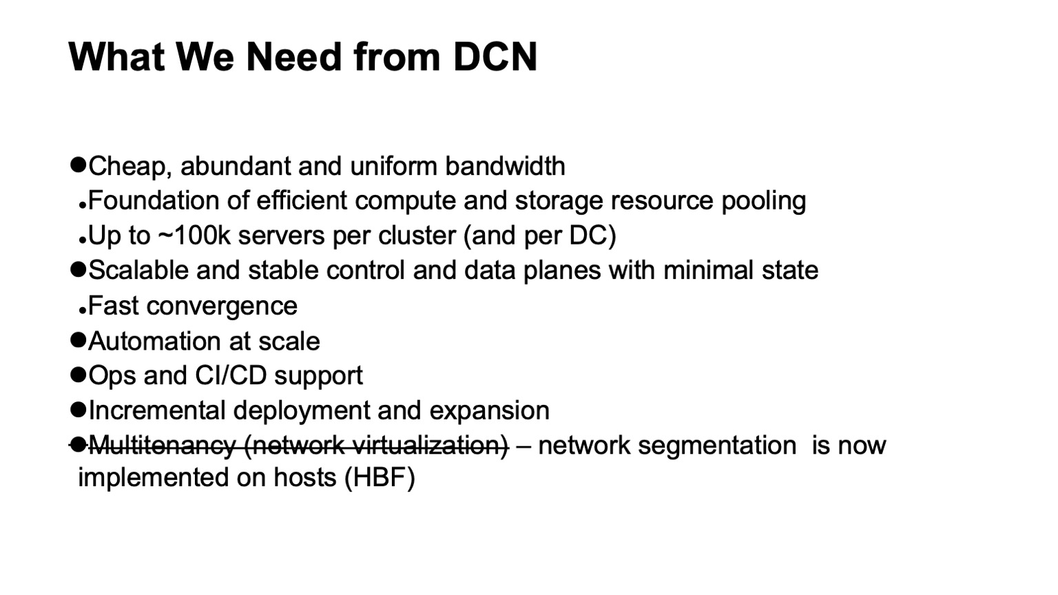
What do we want from a data center network? First of all - a lot of cheap and fairly uniformly distributed bandwidth. Because the network is that substrate through which we can do pooling of resources. The new target size is about 100 thousand servers in one cluster.
Also, of course, we want a scalable and stable control plane, because on such a large infrastructure a lot of headache arises even from just random events, and we do not want the control plane to bring us a headache. At the same time, we want to minimize the state in it. The smaller the condition, the better and more stable everything works, it is easier to diagnose.
Of course, we need automation, because it is impossible to manually manage such an infrastructure, and it was impossible some time ago. Whenever possible, we need operational support and CI / CD support to the extent possible.
With such sizes of data centers and clusters, the task of supporting incremental deployment and expansion without interruption of service has become quite acute. If on clusters the size of a thousand cars is probably close to ten thousand cars, they could still be rolled out as one operation - that is, we are planning to expand the infrastructure, and several thousand machines are added as one operation, then a cluster the size of a hundred thousand cars does not arise just like that, it has been built for some time. And it is desirable that all this time what has already been pumped out, that infrastructure that has been deployed, be available.
And one requirement that we had and left: this is support for multitenancy, that is, virtualization or network segmentation. Now we do not need to do this at the network factory level, because segmentation went to the hosts, and this made scaling very easy for us. Thanks to IPv6 and a large address space, we did not need to use duplicate addresses in the internal infrastructure, all addressing was already unique. And due to the fact that we took filtering and network segmentation to hosts, we do not need to create any virtual network entities in data center networks.
A very important thing is that we do not need. If some functions can be removed from the network, this greatly simplifies life, and, as a rule, expands the choice of available equipment and software, and greatly simplifies diagnostics.
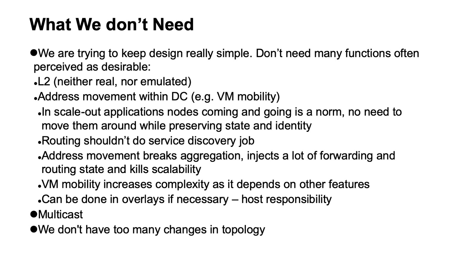
So, what do we not need, what have we been able to refuse, not always with joy at the moment when this happened, but with great relief, when the process was completed?
First of all, the rejection of L2. We do not need L2 either real or emulated. Not used to a large extent due to the fact that we control the application stack. Our applications are scaled horizontally, they work with L3 addressing, they don’t really worry that some particular instance is off, they just roll out a new one, it does not need to roll out on the old address, because there is a separate level of service discovery and monitoring of machines located in the cluster . We do not transfer this task to the network. The task of the network is to deliver packets from point A to point B.
Also, we have no situations where addresses move within the network, and this needs to be monitored. In many designs, this is usually needed to support VM mobility. We do not use the mobility of virtual machines in the internal infrastructure of exactly the big Yandex, and, in addition, we believe that, even if this is done, this should not happen with network support. If you really need to do this, you need to do this at the host level, and drive the addresses that can migrate into overlays so as not to touch or make too many dynamic changes to the routing system itself underlay (transport network).
Another technology that we do not use is multicast. I can tell you in detail why. This makes life much easier, because if someone dealt with him and watched what exactly the control plane of a multicast looks like - in all installations except the simplest, this is a big headache. And what's more, it's hard to find a well-functioning open source implementation, for example.
Finally, we design our networks so that they do not have too many changes. We can expect that the flow of external events in the routing system is small.
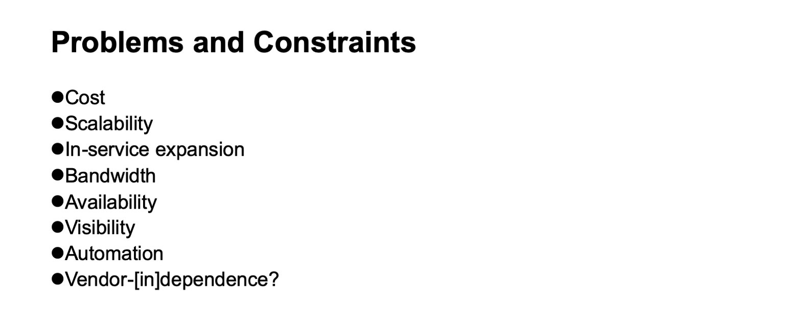
What problems arise and what limitations should be taken into account when we develop a data center network? Cost of course. Scalability, to what level we want to grow. The need for expansion without stopping the service. Bandwidth availability. The visibility of what is happening on the network, for monitoring systems, for operational teams. Support for automation - again, as much as possible, since different tasks can be solved at different levels, including the introduction of additional layers. Well, not- [if possible] -dependence on vendors. Although in different historical periods, depending on which section to look at, this independence was easier or harder to achieve. If we take a slice of the chips of network devices, then until recently, talk about independence from vendors, if we also wanted chips with high bandwidth, it could be very arbitrary.

What logical topology will we use to build our network? This will be a multi-level Clos. In fact, there are currently no real alternatives. And the Clos topology is good enough, even if we compare it with various advanced topologies, which are now more in the sphere of academic interest, if we have switches with a large radix.
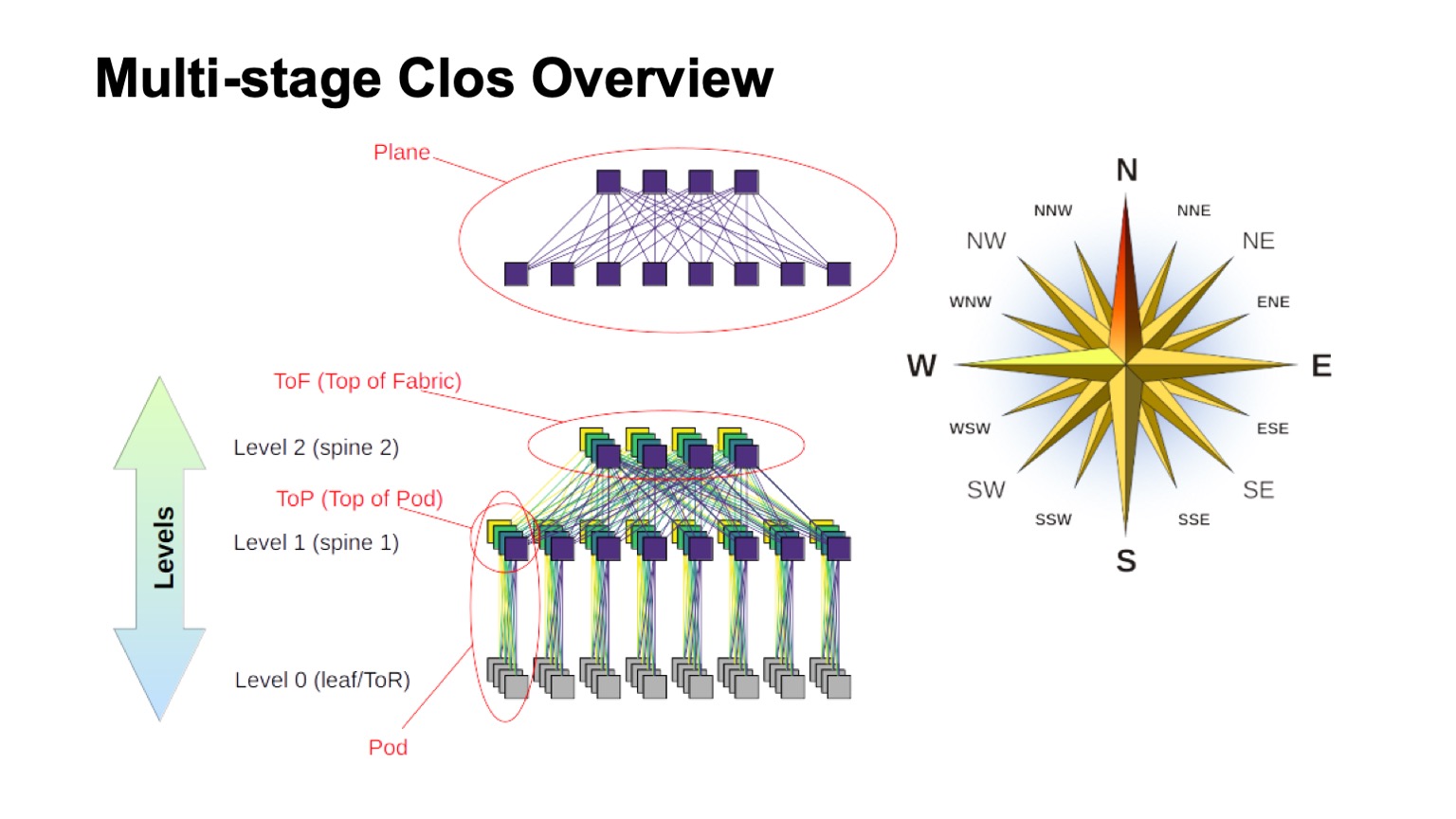
How is the layered Clos network approximately structured and what are the various elements called in it? First of all, the wind rose, to find out where the north, where the south, where the east, where the west. Networks of this type are usually built by those who have very high traffic west - east. As for the remaining elements, the virtual switch assembled from smaller switches is shown at the top. This is the basic idea of recursively building Clos networks. We take elements with some kind of radix and connect them so that what happened can be considered as a larger switch with a radix. If you need even more, the procedure can be repeated.
In cases, for example, with two-level Clos, when it is possible to clearly distinguish components that are vertical in my diagram, they are usually called planes. If we built Clos-with three levels of spine switches (all that are not borderline and not ToR-switches and which are used only for transit), then the planes would look more complicated, two-level look like that. The block of ToR or leaf switches and the associated first level spine switches we call Pod. Spine level 1 switches at the top of the Pod are the top of the Pod, the top of the Pod. The switches that are located at the top of the entire factory are the top layer of the factory, Top of fabric.

Of course, the question arises: Clos-networks have been built for some time, the idea itself generally comes from the days of classical telephony, TDM-networks. Maybe something better appeared, maybe you can do something better somehow? Yes and no. Theoretically, yes, in practice, in the near future, definitely not. Because there are a number of interesting topologies, some of them are even used in production, for example, Dragonfly is used in HPC applications; There are also interesting topologies such as Xpander, FatClique, Jellyfish. If you look at reports at conferences such as SIGCOMM or NSDI recently, you can find a fairly large number of papers on alternative topologies that have better properties (one or the other) than Clos.
But all of these topologies have one interesting property. It prevents their implementation in the networks of data centers, which we are trying to build on commodity hardware and which cost reasonably reasonable money. In all of these alternative topologies, most of the band, unfortunately, is not accessible via the shortest paths. Therefore, we immediately lose the ability to use the traditional control plane.
Theoretically, the solution to the problem is known. These are, for example, modifications of link state using the k-shortest path, but, again, there are no protocols that would be implemented in production and massively available on equipment.
Moreover, since most of the capacity is not accessible by the shortest paths, we need to modify not only the control plane so that it selects all these paths (and, by the way, this is a much larger state in the control plane). We still need to modify the forwarding plane, and, as a rule, at least two additional features are required. This is an opportunity to make all decisions about forwarding packages one-time, for example, on a host. This is actually source routing, sometimes in the literature on interconnection networks this is called all-at-once forwarding decisions. And adaptive routing is already a function that we need on network elements, which boils down, for example, to the fact that we select the next hop based on information about the least load on the queue. As an example, other options are possible.
Thus, the direction is interesting, but, alas, we cannot apply it right now.

Okay, settled on the logical topology of Clos. How will we scale it? Let's see how it works and what can be done.

In the Clos network there are two main parameters that we can somehow vary and get certain results: radix elements and the number of levels in the network. I schematically depict how one and the other affects the size. Ideally, we combine both.
It can be seen that the total width of the Clos network is a product of all levels of spine switches of the southern radix, how many links we have down, how it branches. This is how we scale the size of the network.
As for capacity, especially on ToR switches, there are two scaling options. Either we can, while maintaining the general topology, use faster links, or we can add more planes.
If you look at the detailed version of the Clos network (in the lower right corner) and return to this picture with the Clos network below ...
... then this is exactly the same topology, but on this slide it is collapsed more compactly and the factory planes are superimposed on each other. This is the same.

What does scaling a Clos network look like in numbers? Here I have data on what maximum width a network can get, what maximum number of racks, ToR-switches or leaf-switches, if they are not in racks, we can get depending on what radix of switches we use for spines levels and how many levels we use.
It shows how many racks we can have, how many servers and how much all this can consume at the rate of 20 kW per rack. A little earlier, I mentioned that we aim at a cluster size of about 100 thousand servers.
It can be seen that in this whole construction two and a half options are of interest. There is an option with two layers of spines and 64-port switches, which is a bit short. Then, perfectly fitting options for 128-port (with a 128 radix) spine switches with two levels, or switches with a 32 radix with three levels. And in all cases where there are more radix and more levels, you can make a very large network, but if you look at the expected consumption, as a rule, there are gigawatts. You can lay the cable, but we are unlikely to get so much electricity on one site. If you look at statistics, public data on data centers - very few data centers can be found for an estimated capacity of more than 150 MW. What’s more - as a rule, data center campuses, several large data centers located fairly close to each other.
There is another important parameter. If you look at the left column, usable bandwidth is listed there. It is easy to notice that in a Clos network, a significant part of the ports is spent on connecting the switches to each other. Usable bandwidth is what you can give out, towards the servers. Naturally, I’m talking about conditional ports and about the strip. As a rule, links within the network are faster than links towards the servers, but per unit of band, as far as we can give it out to our server equipment, there are still some more bands within the network itself. And the more levels we do, the greater the unit costs to provide this strip to the outside.
Moreover, even this extra band is not exactly the same. While the spans are short, we can use something like DAC (direct attach copper, that is, twinax cables), or multimode optics, which cost even more or less reasonable money. As soon as we switch to spans more authentically - as a rule, this is single mode optics, and the cost of this additional band increases markedly.
And again, returning to the previous slide, if we make a Clos network without re-subscribing, then it’s easy to look at the diagram, see how the network is built - adding each level of spine switches, we repeat the entire strip that was below. Plus the level - plus the whole same band, as many as there were at the previous level, ports on the switches, as many transceivers. Therefore, the number of levels of spine switches is very desirable to minimize.
Based on this picture, it is clear that we really want to build on something like switches with a 128 radix.
, , .
, ? , - . , . , . , . , , , , . ( ), control plane , , , , . , , .
, , , SerDes- — - . forwarding . , , , , , Clos-, . .
, , . , , , , , , , , , .

— , . , , . , , , - , . , , , , .
, , , . -, , . , , 128 , .
, , , data plane. . , , . , , , . , , , , 128 , . . . .
, - , . ( ), , — ToR- leaf-, . - , , , , - . , , , - .

, , .

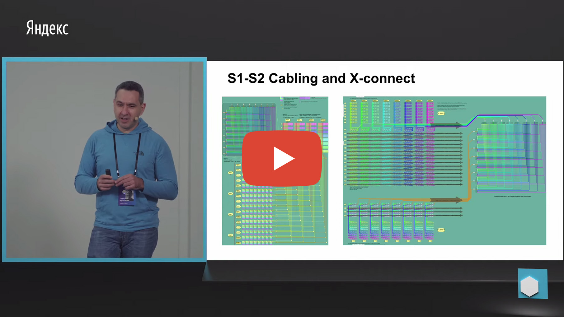
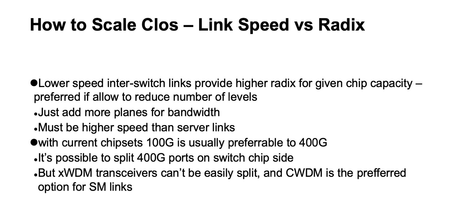
? . , , , : leaf-, 1, 2. , — twinax, multimode, single mode. , , , , , .
. , , multimode , , , 100- . , , , single mode , , single mode, - CWDM, single mode (PSM) , , , .
: , 100 425 . SFP28 , QSFP28 100 . multimode .
- , - , - - . , . , - Pods twinax- ( ).
, , , CWDM. .
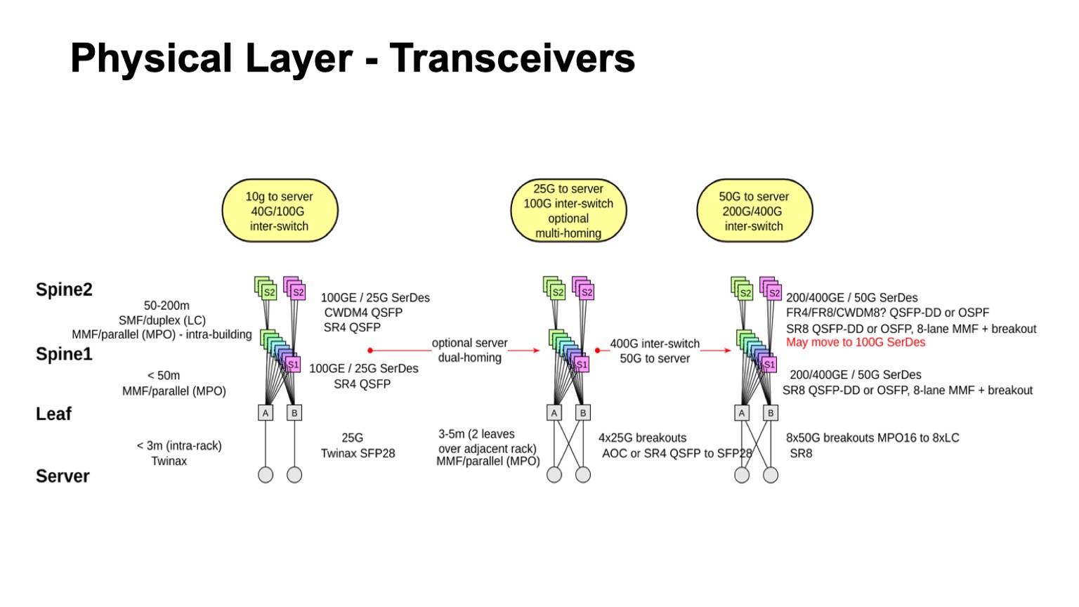
, , . , , 50- SerDes . , , 400G, 50G SerDes- , 100 Gbps per lane. , 50 100- SerDes 100 Gbps per lane, . , 50G SerDes , , , 100G SerDes . - , , .
. , 400- 200- 50G SerDes. , , , , , , . 128. , , , , .
, , . , , , , , 100- , .

— , . , . leaf- — , . , , — .
, , , -. , , - -, . . , , , . - -, -, , , , . : . - , « », Clos-, . , , .
. - , , , , -2-.
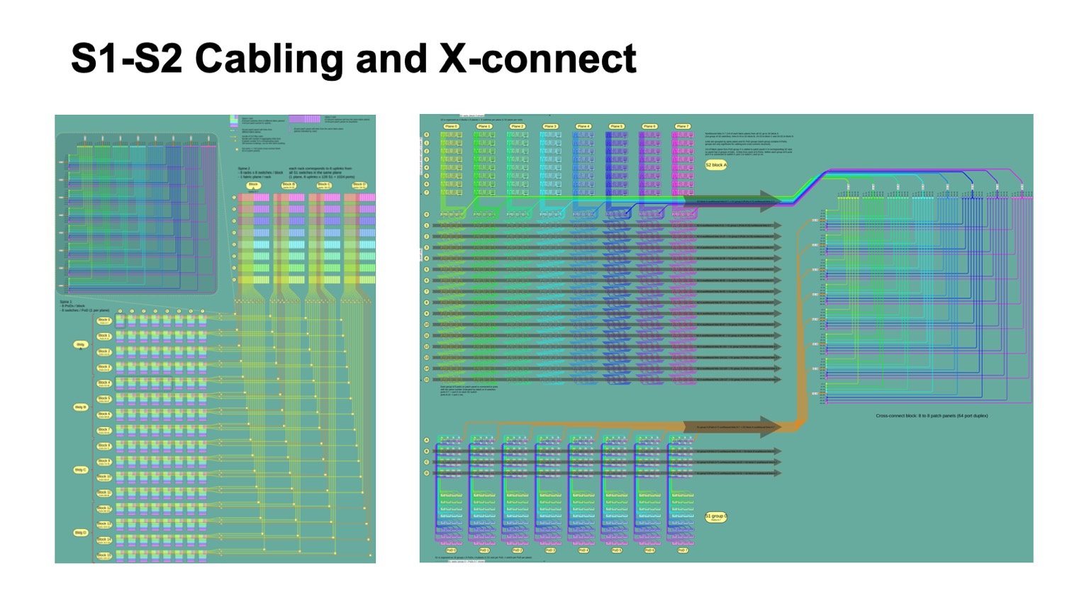
. , - 512 512 , , , -2. Pods -1, -, -2.

Here is how it looks. -2 () -. , . -, . , , .

: , . control plane-? , - , link state , , , , . , — , link state . , , , , fanout, control plane . link state .
— BGP. , RFC 7938 BGP -. : , , , path hunting. , , , valley free. , , , . , , . . .
, , BGP. eBGP, link local, : ToR, -1- Pod, Top of Fabric. , BGP , .

, , , , control plane. L3 , , . — , , , multi-path, multi-path , , , . , , , , , . , multi-path, ToR-.
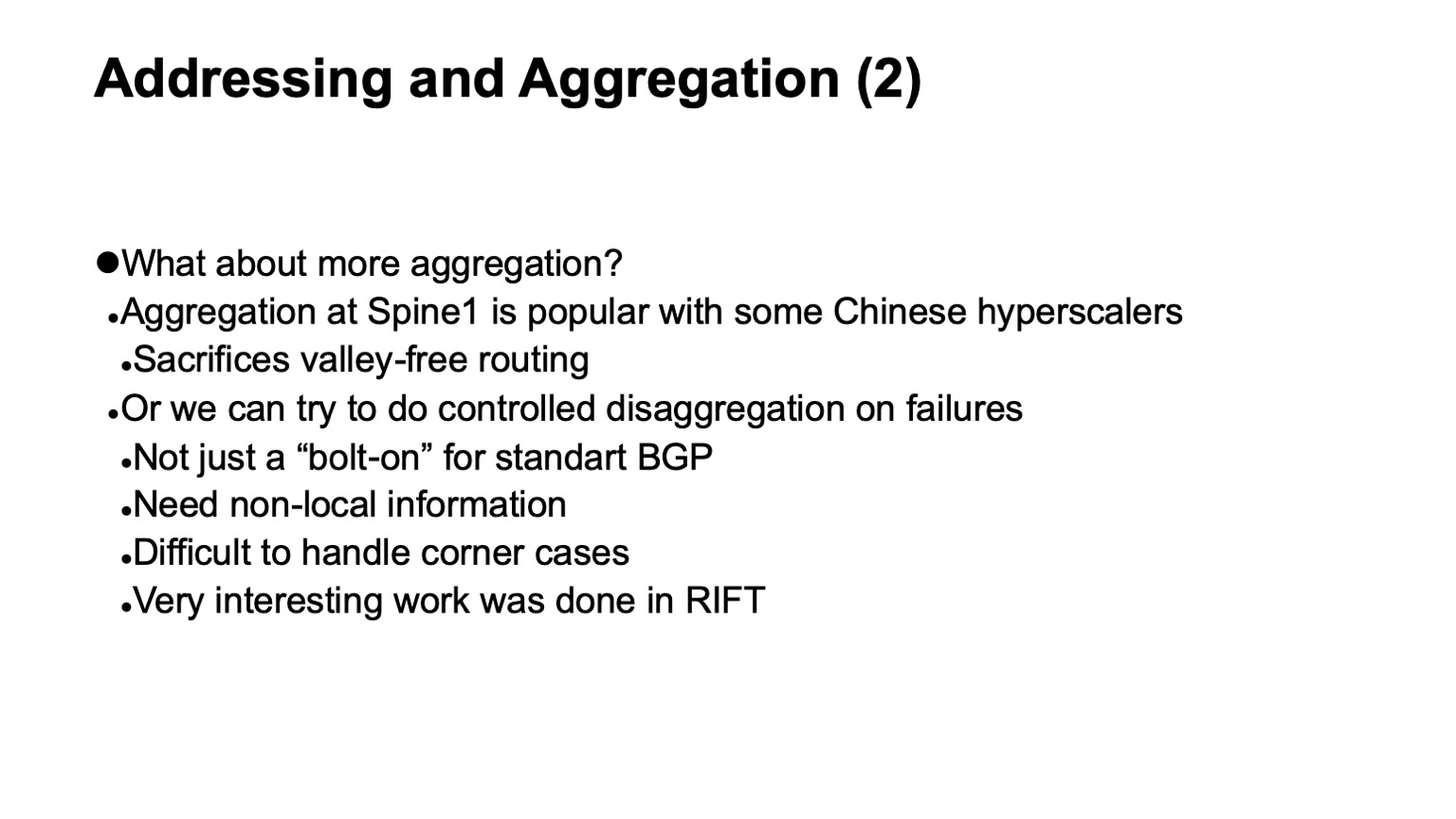
, , — . , , , , BGP, . , corner cases , BGP .
RIFT, .
— , data plane , . : ECMP , Next Hop.
, , Clos- , , , , , . , ECMP, single path-. Things are good. , Clos- , Top of fabric, , . , , . , ECMP state.
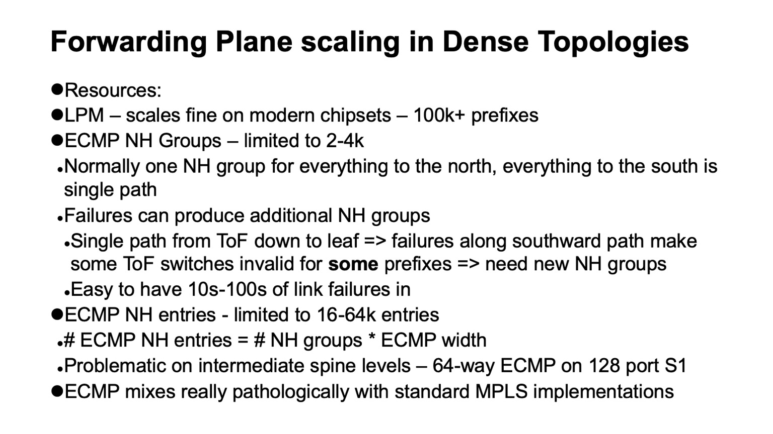
data plane ? LPM (longest prefix match), , 100 . Next Hop , , 2-4 . , Next Hops ( adjacencies), - 16 64. . : MPLS -? , .

. , . white boxes MPLS. MPLS, , , , ECMP. And that's why.

ECMP- IP. Next Hops ( adjacencies, -). , -, Next Hop. IP , , Next Hops.

MPLS , . Next Hops . , , .
, 4000 ToR-, — 64 ECMP, -1 -2. , , ECMP-, ToR , Next Hops.
, Segment Routing . Next Hops. wild card: . , .
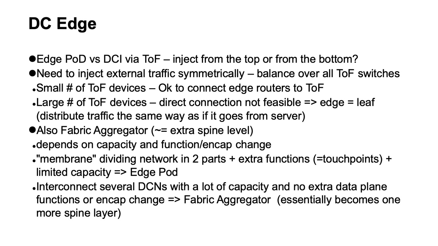
, - . ? Clos- . , Top of fabric. . , , Top of fabric, , , . , , , , .
— . , Clos- , , , ToR, Top of fabric , . Pod, Edge Pod, .
. , , Facebook. Fabric Aggregator HGRID. -, -. , . , touch points, . , , -. , - , , . , , . overlays, .

? — CI/CD-. , , , . , , . , , .
, . . — .
. , RIFT. congestion control , , , , RDMA .
, , , , overhead. — HPC Cray Slingshot, commodity Ethernet, . overhead .

Everything should be done as simple as possible, but not simpler. Complexity is the enemy of scalability. Simplicity and regular structures are our friends. If you can do scale out somewhere, do it. And in general, it’s great to be engaged in network technologies now. A lot of interesting things are happening. Thanks.