⛩️ 🧀 🈺 Introduction to Functional Dependencies 🧑🏿‍🤝‍🧑🏻 ⛹🏽 👨🏾‍🤝‍👨🏻

In this article we will talk about functional dependencies in databases - what it is, where it is applied and what algorithms exist for their search.

We will consider functional dependencies in the context of relational databases. Speaking very rudely, in such databases information is stored in the form of tables. Further, we use approximate concepts, which in a strict relational theory are not interchangeable: we will call the table itself a relation, columns - attributes (their set - relationship scheme), and a set of row values on a subset of attributes - a tuple.

For example, in the table above, (Benson, M, M organ ) is a tuple of attributes (Patient, Gender, Doctor) .

More formally, this is written as follows:

t_{1}

$t_ {1}$ [ Patient, Paul, Doctor ] = (Benson, M, M organ) .

Now we can introduce the concept of functional dependence (FZ):

Definition 1. The relation R satisfies the federal law X → Y (where X, Y ⊆ R) if and only if for any tuples

$t_ {1}$ ,

$t_ {2}$ ∈ R holds: if

$t_ {1}$ [X] =

$t_ {2}$ [X] then

$t_ {1}$ [Y] =

$t_ {2}$ [Y]. In this case, it is said that X (a determinant, or a defining set of attributes) functionally defines Y (a dependent set).

In other words, the presence of the Federal Law X → Y means that if we have two tuples in R and they coincide in the attributes of X , then they will also coincide in the attributes of Y.

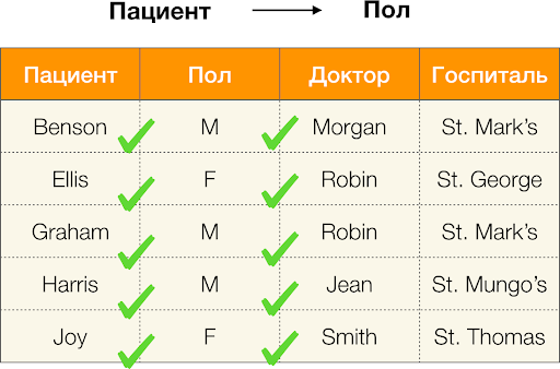
And now in order. Consider the Patient and Gender attributes for which we want to know whether there are dependencies between them or not. For so many attributes, the following dependencies may exist:

Patient → Gender
Gender → Patient

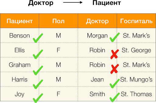
According to the definition above, in order to maintain the first dependence, only one value of the Gender column must correspond to each unique value of the Patient column. And for the sample table this is true. However, this does not work in the opposite direction, that is, the second dependence is not fulfilled, and the Paul attribute is not a determinant for the Patient . Similarly, if you take the dependence Doctor → Patient , you can see that it is violated, since the Robin value for this attribute has several different values - Ellis and Graham .

Thus, functional dependencies make it possible to determine the existing relationships between sets of table attributes. Henceforth, we will consider the most interesting relationships, or rather X → Y such that they are:

nontrivial, that is, the right side of the dependence is not a subset of the left (Y ̸⊆ X) ;
minimal, that is, there is no such dependence Z → Y such that Z ⊂ X.

The dependencies considered up to this point were strict, that is, they did not include any violations on the table, but besides them there are also those that allow some inconsistency between the values of the tuples. Such dependencies are placed in a separate class, called approximate, and allowed to be violated on a certain number of tuples. This amount is controlled by the maximum emax error indicator. For example, the proportion of error

e_{m a x}

$e_ {max}$ = 0.01 may mean that the dependence can be violated by 1% of the available tuples on the considered set of attributes. That is, for 1000 records, a maximum of 10 tuples can violate the Federal Law. We will consider a slightly different metric based on pairwise-different values of the compared tuples. For the dependence X → Y on the relation r, it is considered as follows:

e (X \ rightarrow Y, r) = \ frac {| \ {(t_1, t_2) \ in r ^ 2 \ | \ t_1 [X] = t_2 [X] \ wedge t_1 [Y] \ neq t_2 [Y] \} |} {| r ^ 2 | - | r |}

$e (X \ rightarrow Y, r) = \ frac {| \ {(t_1, t_2) \ in r ^ 2 \ | \ t_1 [X] = t_2 [X] \ wedge t_1 [Y] \ neq t_2 [Y] \} |} {| r ^ 2 | - | r |}$

We calculate the error for Doctor → Patient from the example above. We have two tuples, the values of which differ on the Patient attribute, but coincide on the Doctor :

t_{1}

$t_ {1}$ [ Doctor, Patient ] = ( Robin, Ellis ) and

t_{2}

$t_ {2}$ [ Doctor, Patient ] = ( Robin, Graham ). Following the definition of error, we must take into account all conflicting pairs, which means there will be two: (

t_{1}

$t_ {1}$ ,

t_{2}

$t_ {2}$ ) and its inversion (

t_{2}

$t_ {2}$ ,

t_{1}

$t_ {1}$ ) Substitute in the formula and get:

f r a c 2 5^{2} - 5 = 0.1

$\ frac {2} {5 ^ 2 - 5} = 0.1$

Now let's try to answer the question: “Why is it all?”. In fact, Federal Laws are different. The first type is those dependencies that are determined by the administrator at the database design stage. Usually they are few, they are strict, and the main application is data normalization and the design of the relationship scheme.

The second type is dependencies representing “hidden” data and previously unknown relationships between attributes. That is, such dependencies were not thought at the time of design and are already found for the existing data set, so that then, based on the set of identified Federal Laws, any conclusions about the stored information can be made. It is with such dependencies that we are working. They are engaged in a whole field of mining data with various search techniques and algorithms built on their basis. Let's understand how the found functional dependencies (exact or approximate) in any data can be useful.

Today, data cleansing is among the main areas of application of dependencies. It involves the development of processes for identifying "dirty data" with their subsequent correction. Bright representatives of "dirty data" are duplicates, data errors or typos, missing values, outdated data, extra spaces and the like.

Example data error:

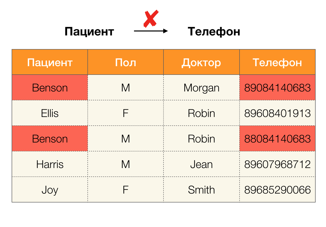
Example duplicates in data:

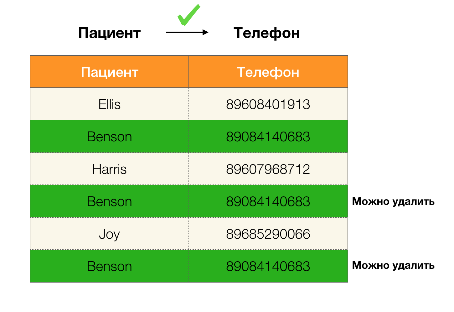
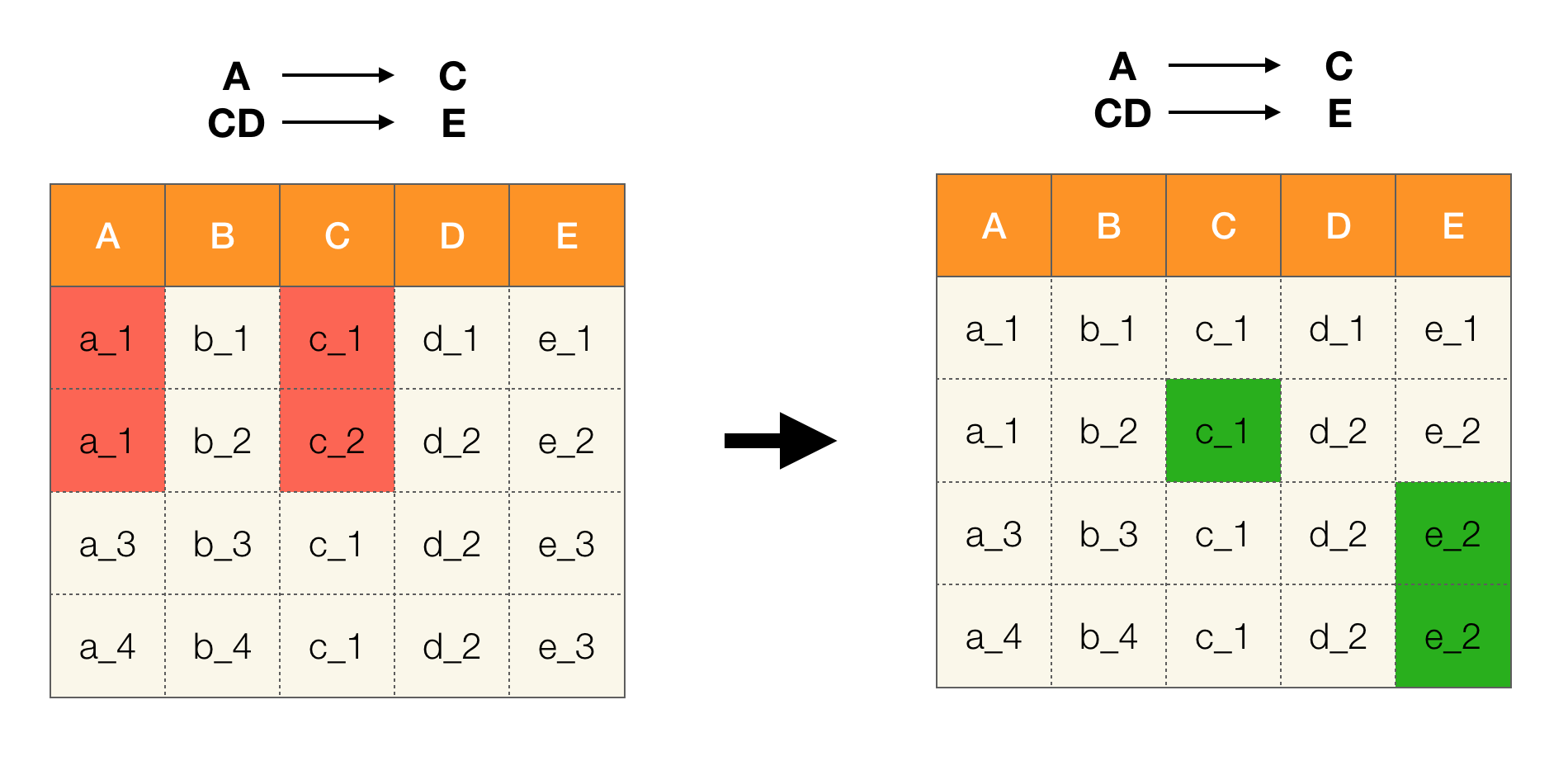
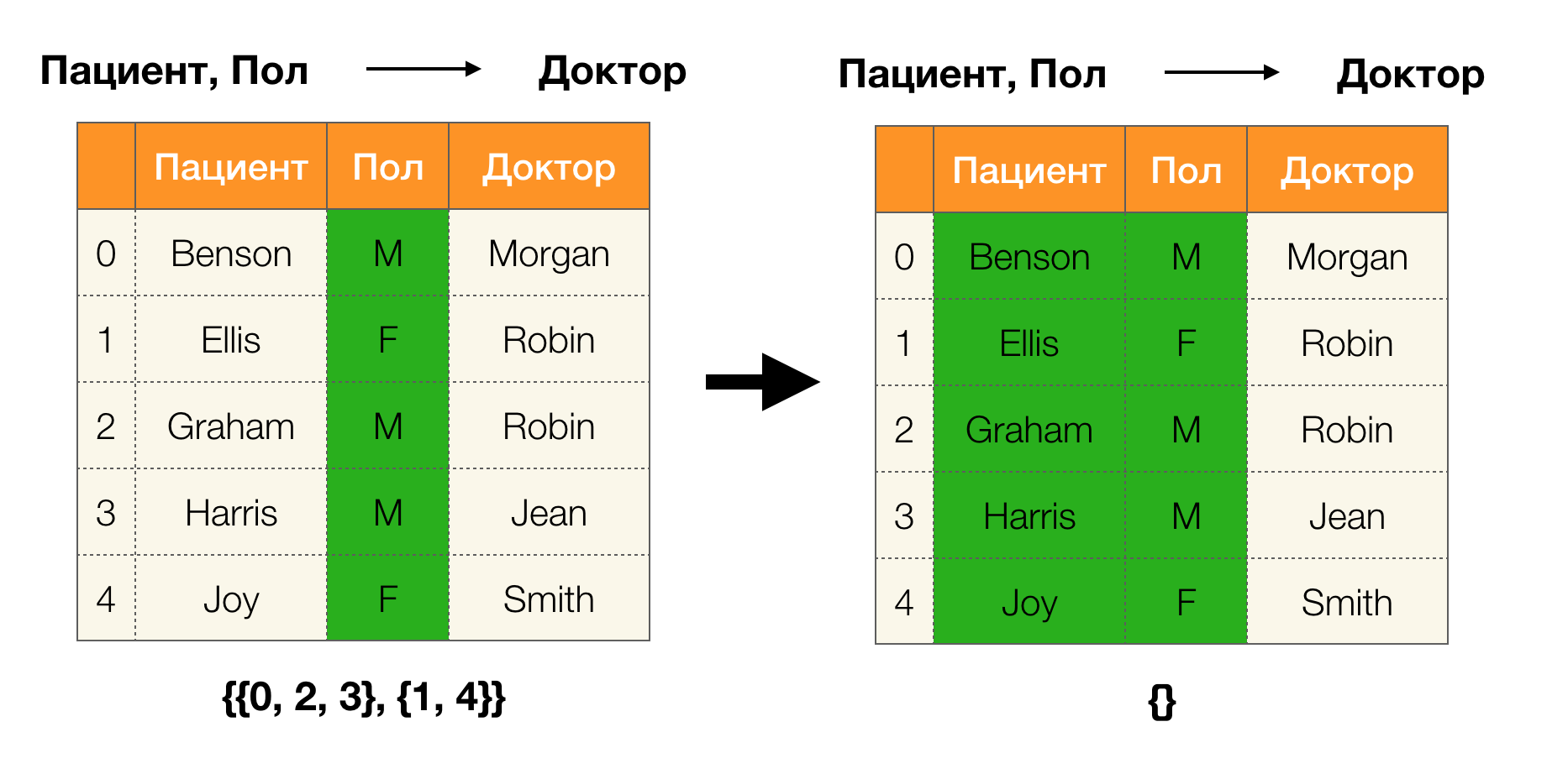
For example, we have a table and a set of Federal Laws that must be executed. Data cleaning in this case involves changing the data so that the Federal Laws are correct. In this case, the number of modifications should be minimal (for this procedure there are algorithms on which we will not focus in this article). The following is an example of such data conversion. On the left is the initial relation, in which, obviously, the necessary federal laws are not fulfilled (an example of violation of one of the federal laws is highlighted in red). On the right is an updated relation in which the green cells show the changed values. After such a procedure, the necessary dependencies began to hold.

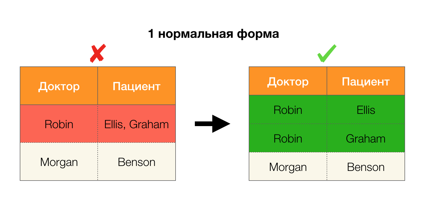
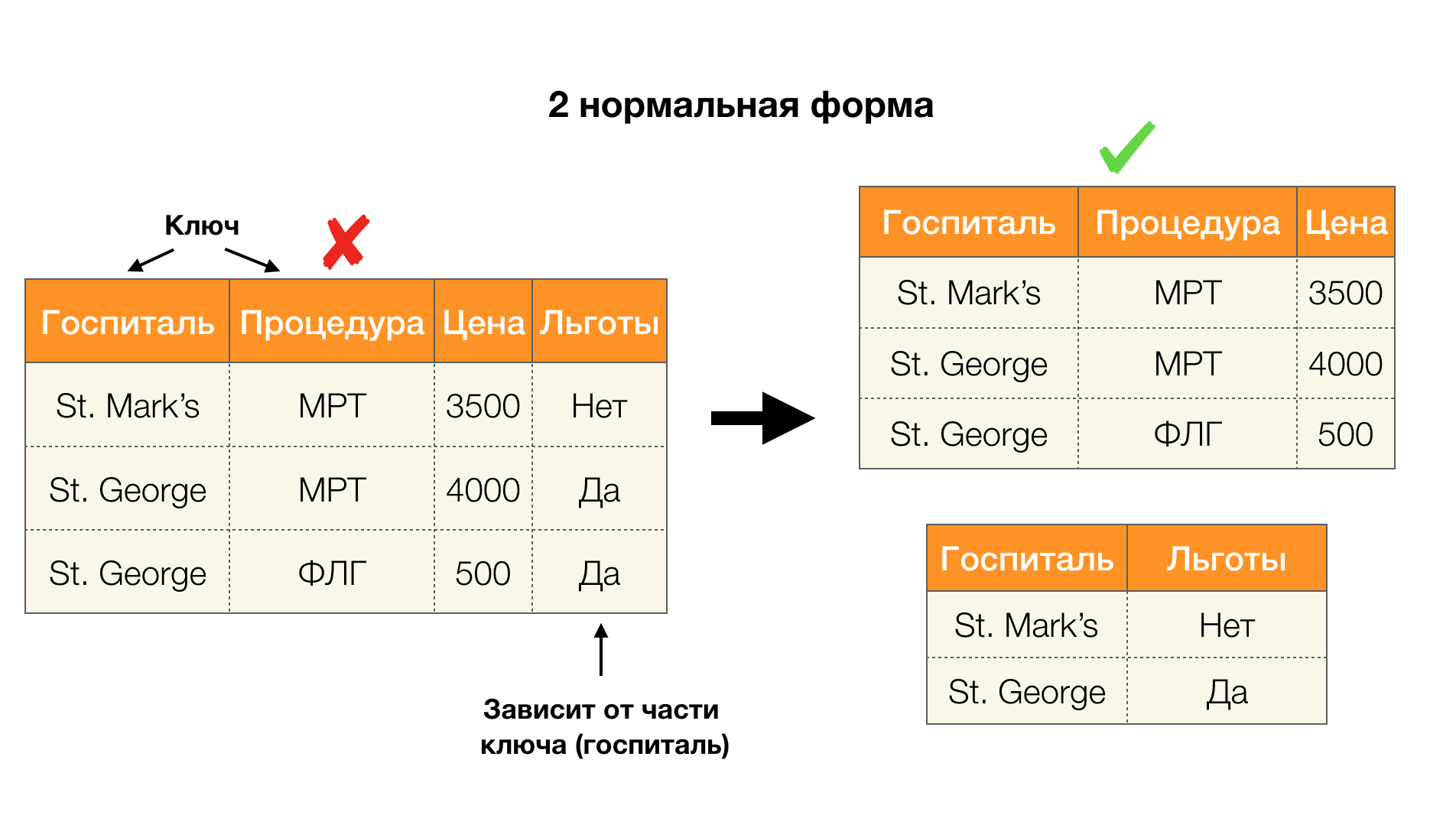
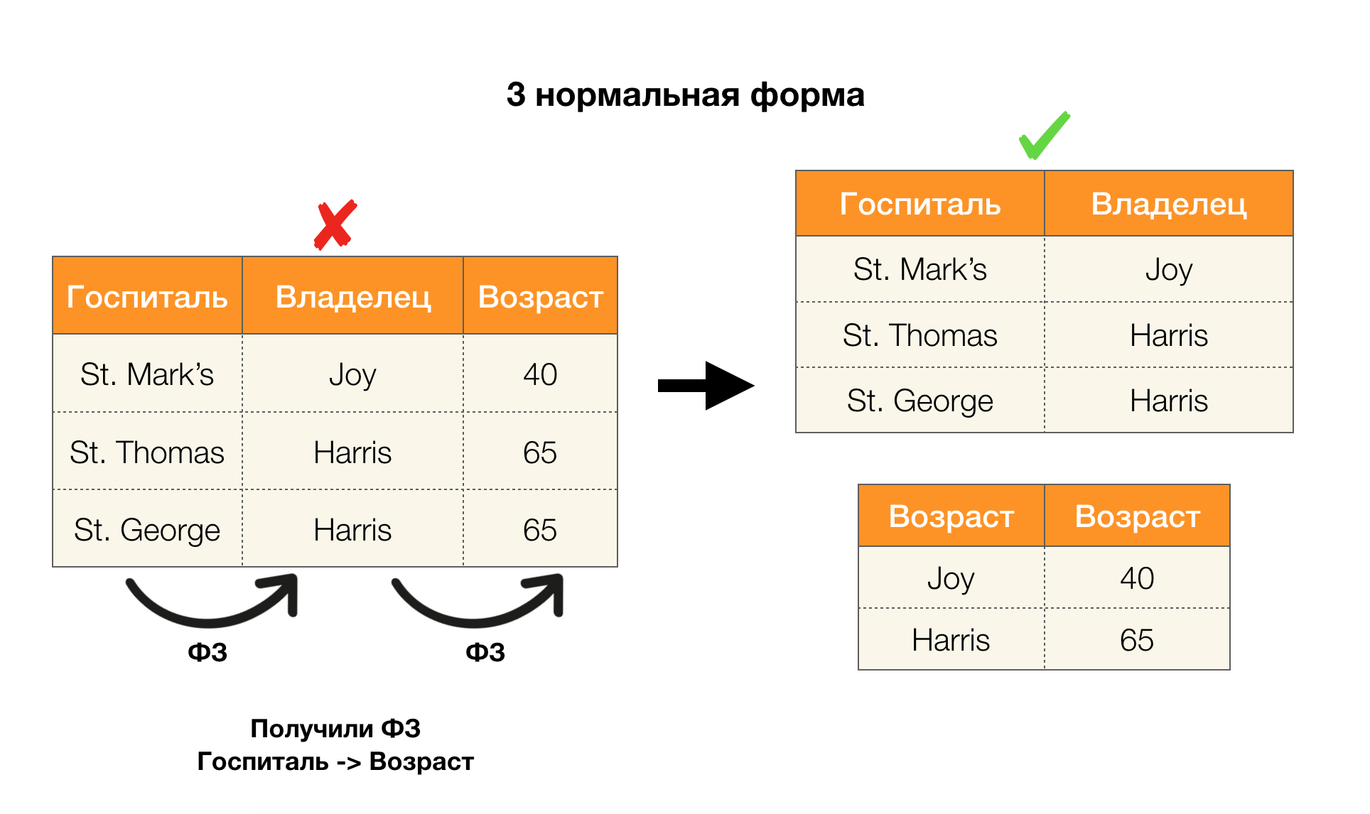
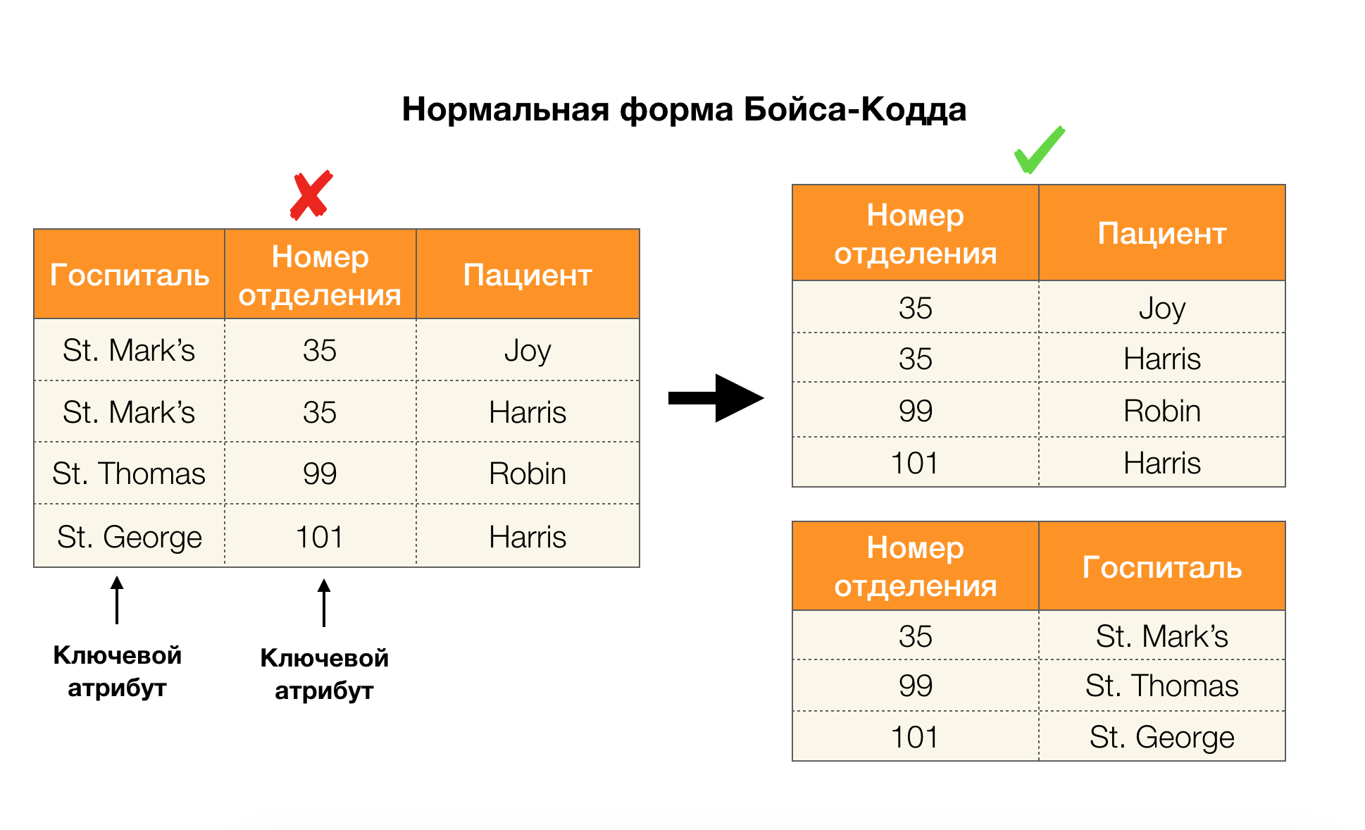
Another popular application is database design. It is worth recalling about normal forms and normalization. Normalization is the process of bringing a relationship into line with a certain set of requirements, each of which is determined in its own way by a normal form. We will not write down the requirements of various normal forms (this is done in any book on the DB course for beginners), but we only note that each of them in its own way uses the concept of functional dependencies. Indeed, Federal Laws are inherently integrity constraints that are taken into account when designing a database (in the context of this task, Federal Laws are sometimes called superkeys).

Consider their application for the four normal forms in the picture below. Recall that the normal Boyce-Codd form is more stringent than the third form, but less stringent than the fourth. We do not consider the latter yet, since its formulation requires an understanding of multi-valued dependencies, which are not of interest to us in this article.

Another area in which the dependences have found their application is the reduction of the dimension of the space of attributes in such problems as the construction of a naive Bayesian classifier, the allocation of significant features and the reparametrization of the regression model. In the original articles, this problem is called the definition of redundant features and feature relevancy [5, 6], and it is solved with the active use of database concepts. With the advent of such works, we can say that today there is a request for solutions that allow combining the database, analytics, and implementation of the above optimization problems into one tool [7, 8, 9].

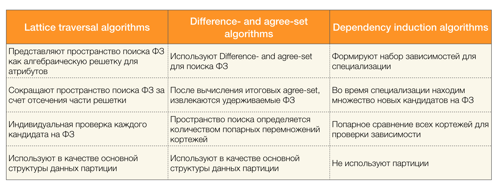
There are many algorithms (both modern and not very) to search for the Federal Law in a data set. Such algorithms can be divided into three groups:

Algorithms using traversal of algebraic lattices (Lattice traversal algorithms)
Algorithms based on the search for consistent values (Di ﬀ erence- and agree-set algorithms)
Pairwise Comparison Algorithms (Dependency induction algorithms)

A brief description of each type of algorithm is presented in the table below:

More details on this classification can be read [4]. Below are examples of algorithms for each type:

Currently, new algorithms are appearing that combine several approaches to the search for functional dependencies at once. Examples of such algorithms are Pyro [2] and HyFD [3]. Analysis of their work is expected in the following articles of this series. In this article, we will only analyze the basic concepts and lemma that are necessary for understanding the techniques for detecting dependencies.

Let's start with a simple one - di ﬀ erence- and agree-set, used in the second type of algorithms. Di ﬀ erence-set is a set of tuples that do not match in values, and agree-set, on the contrary, is tuples that match in values. It should be noted that in this case we consider only the left side of the dependence.

Also an important concept that was met above is the algebraic lattice. Since many modern algorithms operate on this concept, we need to have an idea of what it is.

In order to introduce the concept of a lattice, it is necessary to define a partially ordered set (or partially ordered set, for short - poset).

Definition 2. It is said that the set S is partially ordered by the binary relation ⩽ if for any a, b, c ∈ S the following properties are satisfied:

Reflexivity, i.e. a ⩽ a
Antisymmetry, that is, if a ⩽ b and b ⩽ a, then a = b
Transitivity, that is, for a ⩽ b and b ⩽ c it follows that a ⩽ c

Such a relation is called a relation of (non-strict) partial order, and the set itself is called a partially ordered set. Formal notation: ⟨S, ⩽⟩.

As the simplest example of a partially ordered set, we can take the set of all natural numbers N with the usual relation of order ⩽. It is easy to verify that all the necessary axioms are satisfied.

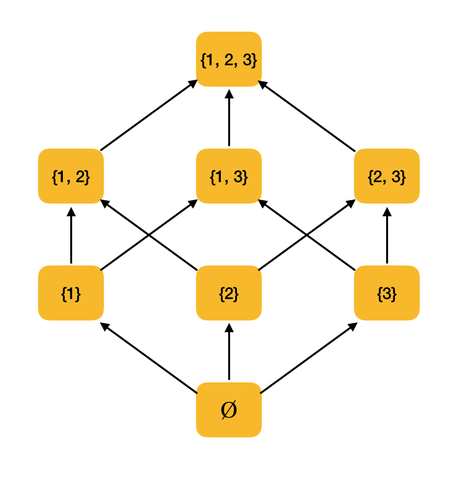
More substantial example. Consider the set of all subsets {1, 2, 3} ordered by the inclusion relation ⊆. Indeed, this relation satisfies all conditions of partial order; therefore, ⟨P ({1, 2, 3}), ⊆⟩ is a partially ordered set. The figure below shows the structure of this set: if from one element you can reach the other element along the arrows, then they are in order relation.

We will need two more simple definitions from the field of mathematics - supremum and infimum.

Definition 3. Let ⟨S, ⩽⟩ be a partially ordered set, A ⊆ S. The upper boundary of A is an element u ∈ S such that ∀x ∈ A: x ⩽ u. Let U be the set of all upper bounds of A. If U has the smallest element, then it is called a supremum and is denoted by sup A.

Similarly, the concept of an exact lower bound is introduced.

Definition 4. Let ⟨S, ⩽⟩ be a partially ordered set, A ⊆ S. The lower boundary of A is an element l ∈ S such that ∀x ∈ A: l ⩽ x. Let L be the set of all lower bounds of A. If L has the largest element, then it is called an infimum and is denoted by inf A.

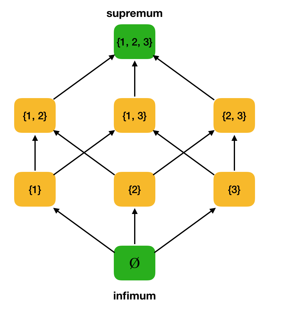
Consider, as an example, the above partially ordered set ⟨P ({1, 2, 3}), and find the supremum and infimum in it:

Now we can formulate the definition of an algebraic lattice.

Definition 5. Let ⟨P, ⩽⟩ be a partially ordered set such that every two-element subset has exact upper and lower bounds. Then P is called an algebraic lattice. Moreover, sup {x, y} is written as x ∨ y, and inf {x, y} is written as x ∧ y.

Let us verify that our working example ⟨P ({1, 2, 3}), ⊆⟩ is a lattice. Indeed, for any a, b ∈ P ({1, 2, 3}), a∨b = a∪b, and a∧b = a∩b. For example, consider the sets {1, 2} and {1, 3} and find their infimum and supremum. If we cross them, we get the set {1}, which will be the infimum. We get the supremum by their union - {1, 2, 3}.

In FD detection algorithms, the search space is often represented in the form of a lattice, where sets of one element (read the first level of the search lattice, where the left part of the dependencies consists of one attribute) are each attribute of the original relationship.

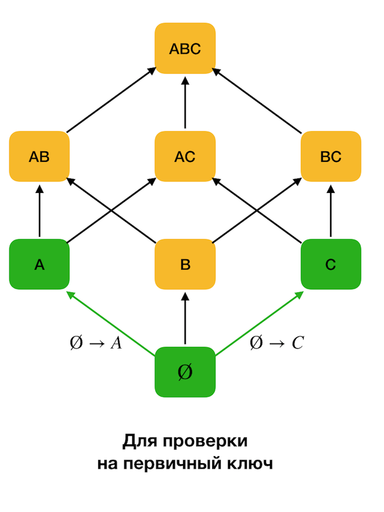
At the beginning, we consider the dependencies of the form → Single attribute. This step allows you to determine which attributes are the primary keys (there are no determinants for such attributes, and therefore the left side is empty). Further, such algorithms move up the lattice. It is worth noting that the lattice can not be bypassed all, that is, if the desired maximum size of the left part is transmitted to the input, the algorithm will not go beyond the level with this size.

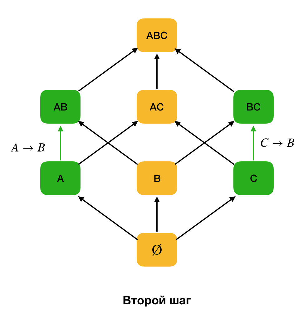
The figure below shows how you can use the algebraic lattice in the search problem for the Federal Law. Here, each edge ( X, XY ) represents a dependence X → Y. For example, we went through the first level and we know that the dependence A → B is kept (we will display this by the green connection between the vertices A and B ). Therefore, when we move up the lattice upwards, we can not check the dependence A, C → B , because it will no longer be minimal. Similarly, we would not check it if the dependence C → B were kept.

In addition, as a rule, all modern FZ search algorithms use such a data structure as a partition (stripped partition [1] in the original source). The formal definition of partition is as follows:

Definition 6. Let X ⊆ R be the set of attributes for the relation r. A cluster is a set of indices of tuples from r that have the same value for X, that is, c (t) = {i | ti [X] = t [X]}. Partition is a set of clusters, excluding clusters of unit length:

\ pi (X): = \ {c (t) | t \ in r \ wedge | c (t) | > 1 \}

$\ pi (X): = \ {c (t) | t \ in r \ wedge | c (t) | > 1 \}$

In simple words, the partition for attribute X is a set of lists, where each list contains line numbers with the same values for X. In modern literature, a structure representing partitions is called a position list index (PLI). Unit length clusters are excluded for PLI compression because they are clusters containing only a record number with a unique value that will always be easy to set.

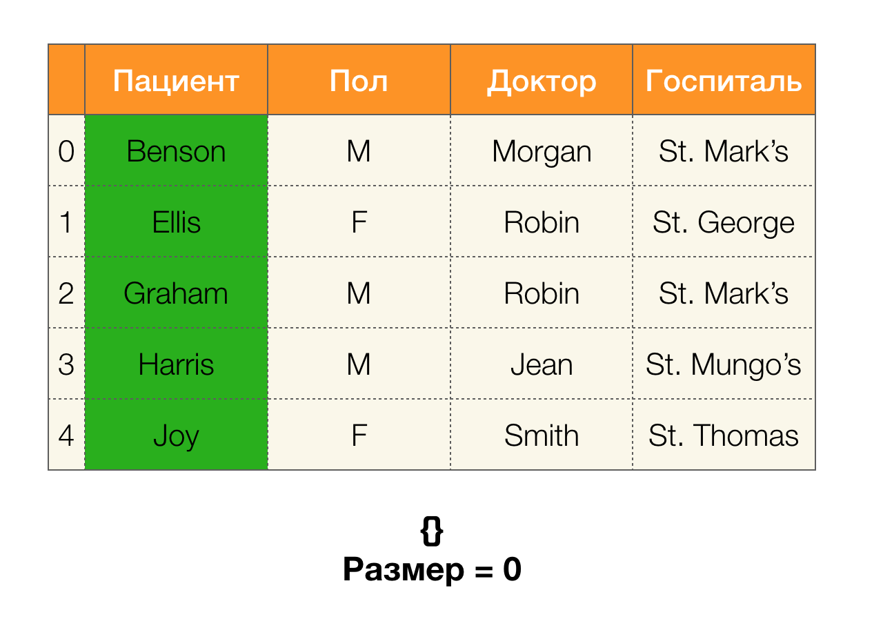
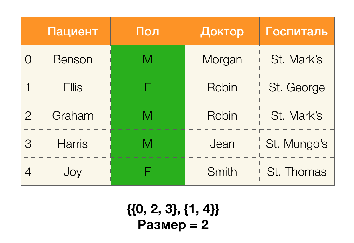
Consider an example. Let's go back to the same table with patients and build partitions for the Patient and Paul columns (a new column appeared on the left, in which the row numbers of the table are marked):

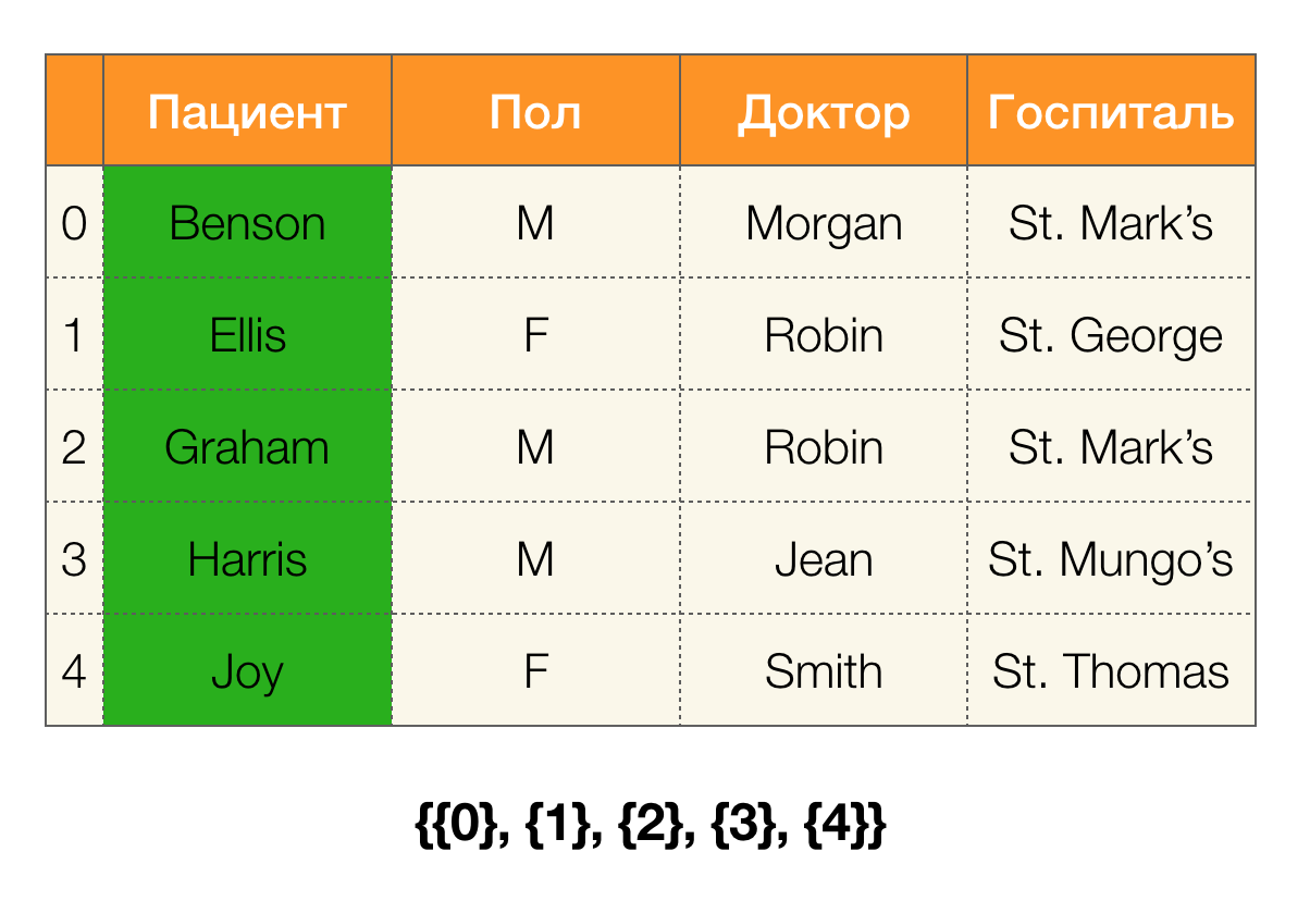
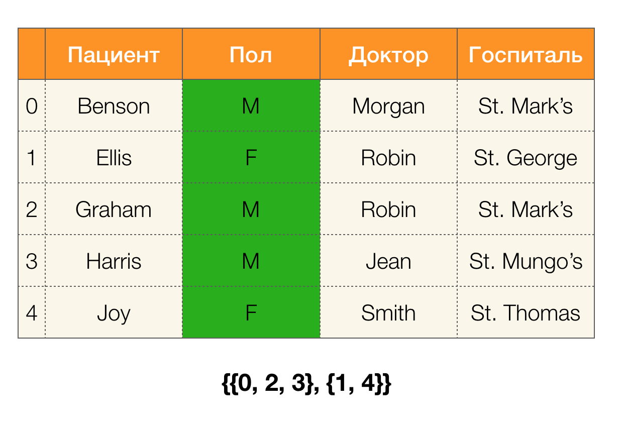
In this case, according to the definition, the partition for the Patient column will actually be empty, since single clusters are excluded from the partition.

Partitions can be obtained by several attributes. And for this there are two ways: going through the table, build a partition at once according to all necessary attributes, or build it using the operation of crossing partitions along a subset of attributes. FZ search algorithms use the second option.

In simple words, to, for example, get a partition by ABC columns, you can take partitions for AC and B (or any other set of disjoint subsets) and intersect them. The operation of intersection of two partitions identifies clusters of the greatest length common to both partitions.

Let's look at an example:

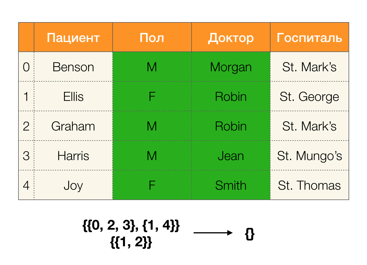
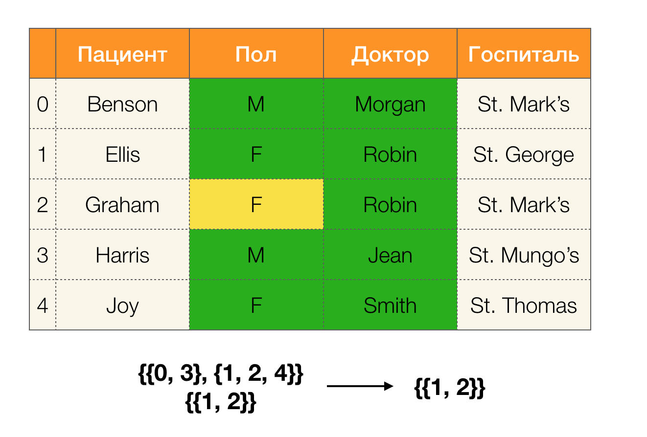
In the first case, we received an empty partition. If you look closely at the table, then indeed, the identical values for the two attributes are not there. If we slightly modify the table (the case on the right), then we already get a nonempty intersection. At the same time, lines 1 and 2 really contain the same values for the attributes Paul and Doctor .

Next, we need such a concept as partition size. Formally:

| \ pi (X) | = | \ {c \ in \ pi (X): | c | > 1 \} |

$| \ pi (X) | = | \ {c \ in \ pi (X): | c | > 1 \} |$

Simply put, the partition size is the number of clusters included in the partition (remember that individual clusters are not included in the partition!):

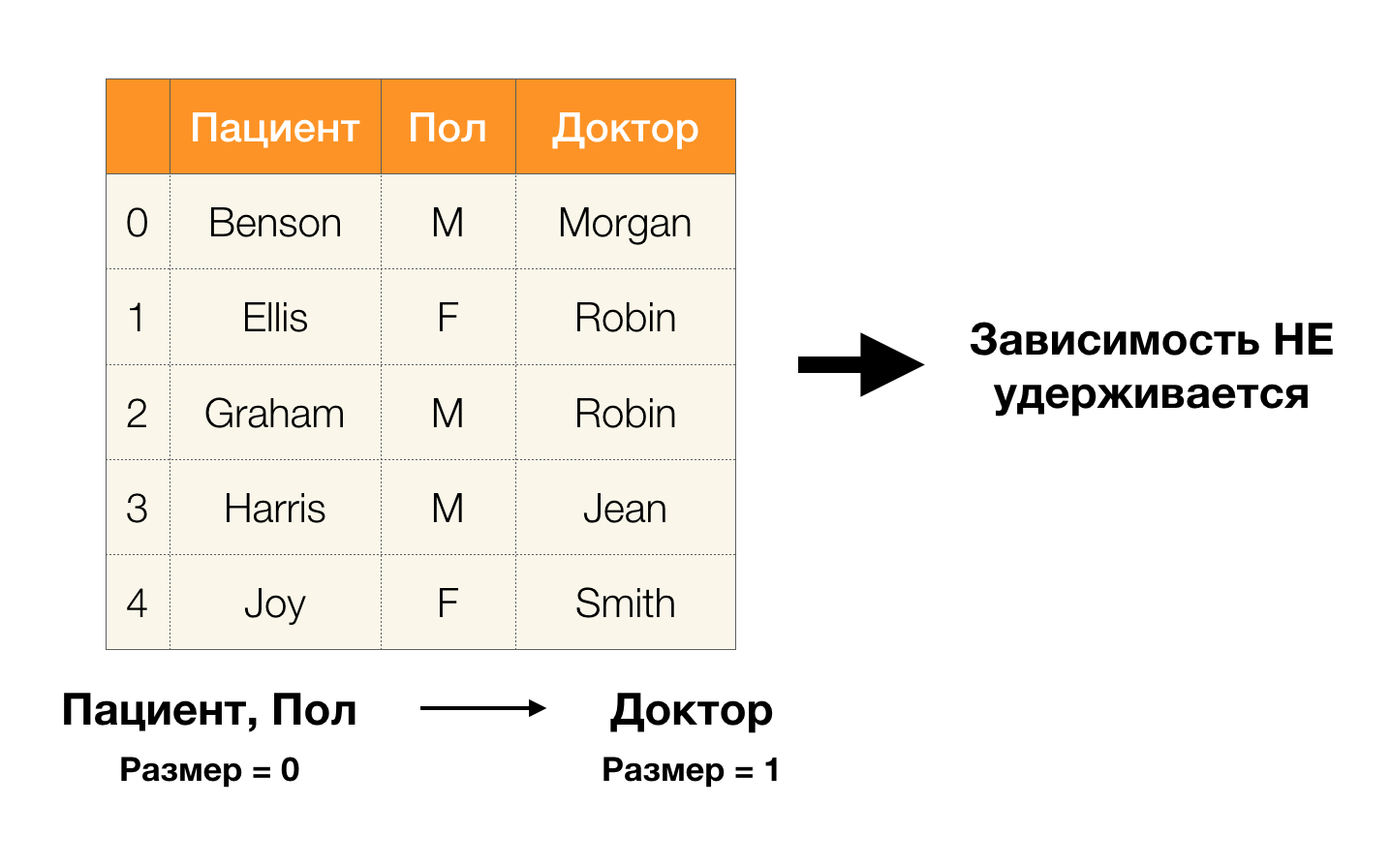
Now we can define one of the key lemmas, which for given partitions allows us to establish whether the dependency is held or not:

Lemma 1 . The dependence A, B → C is held if and only if

| \ pi (AB) | = | \ pi (AB \ cup \ {C \}) |

$| \ pi (AB) | = | \ pi (AB \ cup \ {C \}) |$

According to the lemma, to determine whether a dependency is held, four steps must be performed:

Calculate the partition for the left side of the dependency
Calculate the partition for the right side of the dependency
Calculate the product of the first and second steps
Compare the sizes of partitions obtained in the first and third step

The following is an example of checking whether the dependence is maintained by this lemma:

In this article, we examined concepts such as functional dependence, approximate functional dependence, examined where they are used, as well as what search algorithms for the Federal Law exist. We also examined in detail the basic, but important concepts that are actively used in modern algorithms for searching for Federal Laws.

References to the literature:

Huhtala Y. et al. TANE: An efficient algorithm for discovering functional and approximate dependencies // The computer journal. - 1999. - T. 42. - No. 2. - S. 100-111.
Kruse S., Naumann F. Efficient discovery of approximate dependencies // Proceedings of the VLDB Endowment. - 2018. - T. 11. - No. 7. - S. 759-772.
Papenbrock T., Naumann F. A hybrid approach to functional dependency discovery // Proceedings of the 2016 International Conference on Management of Data. - ACM, 2016 .-- S. 821-833.
Papenbrock T. et al. Functional dependency discovery: An experimental evaluation of seven algorithms // Proceedings of the VLDB Endowment. - 2015. - T. 8. - No. 10. - S. 1082-1093.
Kumar A. et al. To join or not to join ?: Thinking twice about joins before feature selection // Proceedings of the 2016 International Conference on Management of Data. - ACM, 2016 .-- S. 19-34.
Abo Khamis M. et al. In-database learning with sparse tensors // Proceedings of the 37th ACM SIGMOD-SIGACT-SIGAI Symposium on Principles of Database Systems. - ACM, 2018 .-- S. 325-340.
Hellerstein JM et al. The MADlib analytics library: or MAD skills, the SQL // Proceedings of the VLDB Endowment. - 2012. - T. 5. - No. 12. - S. 1700-1711.
Qin C., Rusu F. Speculative approximations for terascale distributed gradient descent optimization // Proceedings of the Fourth Workshop on Data analytics in the Cloud. - ACM, 2015 .-- S. 1.
Meng X. et al. Mllib: Machine learning in apache spark // The Journal of Machine Learning Research. - 2016. - T. 17. - No. 1 .-- S. 1235-1241.

Authors of the article: Anastasia Birillo , researcher at JetBrains Research , student at the CS center and Nikita Bobrov , researcher at JetBrains Research

Introduction to Functional Dependencies

More articles: