
The problem had to be solved. How did Robert decide it? He bought some iron to his computer, connected an outdoor surveillance camera looking over the lawn to it, and then did a somewhat unusual thing, he downloaded the available free Open Source software - a neural network, and began to train her to recognize cats in the camera image. And the task at the beginning seems trivial, because if you learn something and it's easy, it's cats, because cats are littered with the Internet, there are tens of millions of them. If everything was so simple, but things are worse, in real life cats go to crap mostly at night. There are practically no pictures of night cats peeing on the lawn on the Internet. And some of the cats even manage to drink from the irrigation system during work, but still dump it.

Below we provide a description of the project from the author, the English version can be found here .
This project was motivated by two things: the desire to learn more about neural network software and the desire to encourage neighboring cats to hang out somewhere else besides my lawn.
The project includes only three hardware components: the Nvidia Jetson TX1 board, the Foscam FI9800P IP camera and the Particle Photon connected to the relay . The camera is mounted on the side of the house on the side of the lawn. She contacts the WIFI access point followed by Jetson. Particle Photon and relays are installed in the control unit of my irrigation system and connected to a WI-FI access point in the kitchen.
In the process, the camera is configured to monitor changes in the yard. When something changes, the camera transmits a set of 7 images to Jetson, one per second. The Jetson-powered service tracks incoming images, transferring them to Caffe's deep training neural network. If the network detects a cat, Jetson signals to the Particle Photon server in the cloud, which sends a message to Photon. Photon responds by turning on the sprinklers for two minutes.
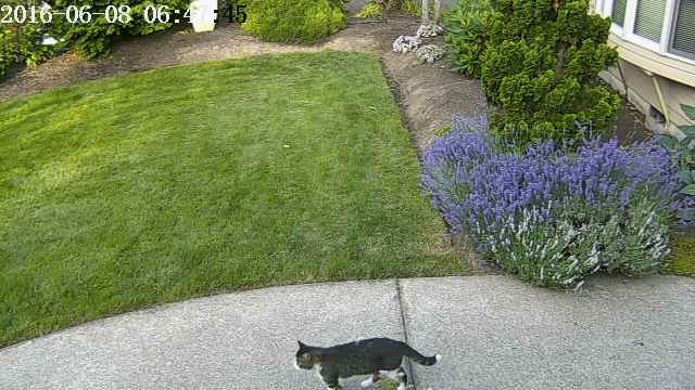
Here the cat went into the frame, turning on the camera:
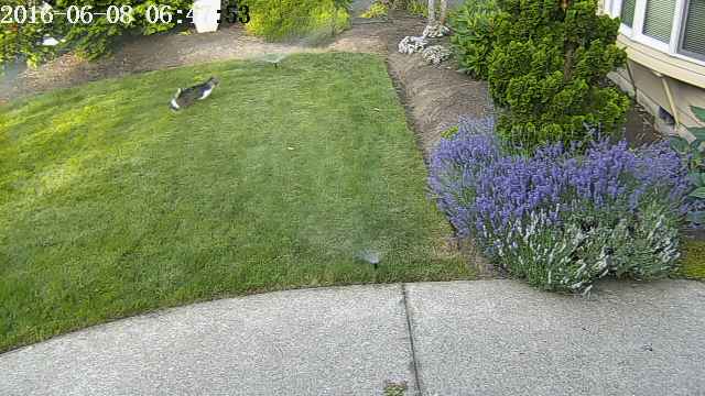
After a few seconds, the cat got out into the middle of the yard, turning on the camera again and activated the sprinklers of the irrigation system:
Camera installation
There was nothing unusual about installing a camera. The only permanent connection is a 12-volt wired connection that goes through a small hole under the ledge. I mounted the camera on a wooden box to capture the front yard with a lawn. A bunch of wires are connected to the camera, which I hid in a box.
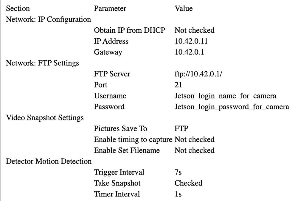
Follow the directions from Foscam to associate it with Jetson's AP (see below). In my setup, Jetson is at 10.42.0.1. I assigned a fixed IP address of 10.42.0.11 to the camera so that it would be easy to find. Once this is done, connect the Windows laptop to the camera and configure the “Warning” parameter to activate the change. Set up upload of 7 images via FTP by warning (alert). Then give it the user ID and password on Jetson. My camera sends 640x360 images via FTP to their home directory.
Below you can see the parameters that were selected for the camera configuration.
Setting up Particle Photon
Photon was easy to set up. I put it in the irrigation control unit.

The black box on the left with the blue LED is a 24 V AC (5 V) converter converted to 5 V DC (DC), purchased on eBay. You can see the white relay on the relay board and the blue connector on the front. Photon itself is on the right. Both are glued to a piece of cardboard to hold them together.
The 5 V output from the converter is connected to the Particle Photon VIN connector. The relay board is mostly analog: it has an open collector NPN transistor with a nominal 3.3 V input to the transistor base and a 3 V relay. The photon controller could not supply enough current to control the relay, so I connected the collector of the transistor input to 5 V through a resistor with a resistance of 15 Ohms and a power of 1/2 W, limiting the current. The relay contacts are connected to the water fan in parallel with the normal control circuit.
Here is the connection diagram:
24VAC converter 24VAC <---> Control box 24VAC OUT
24VAC converter + 5V <---> Photon VIN, resistor to relay board + 3.3V
24VAC converter GND <---> Photon GND, Relay GND
Photon D0 <---> Relay board signal input
Relay COM <---> Control box 24VAC OUT
Relay NO <---> Front yard water valve
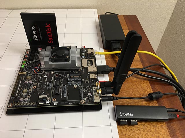
Install Jetson
The only hardware components added to Jetson are a SATA SSD and a small Belkin USB hub. The hub has two wireless keys that connect a keyboard and mouse.
SSD came up without a problem. I reformatted it to EXT4 and installed it as / caffe. I highly recommend deleting all of your project code, git repositories, and application data from the Jetson internal SD card, because it is often easiest to wipe the system during a Jetpack upgrade.
Setting up a wireless access point was pretty simple (true!) If you followed this guide . Just use the Ubuntu menu as indicated, and be sure to add this configuration parameter .
I installed vsftpd as an FTP server . The configuration is largely stock. I did not enable anonymous FTP. I gave the camera a username and password that are no longer used for anything.
I installed Caffe using the JetsonHacks recipe. I believe that there is no longer an LMDB_MAP_SIZE problem in current releases, so try building it before you make any changes. You should be able to run the tests and timing demo mentioned in the JetsonHacks shell script. I am currently using Cuda 7.0, but I am not sure if this is significant at this stage. Use CDNN, it saves a significant amount of memory in these small systems. Once it is built, add the assembly directory to the PATH variable so that scripts can find Caffe. Also add the Caffe Python lib directory to your PYTHONPATH.
~ $ echo $PATH /home/rgb/bin:/caffe/drive_rc/src:/caffe/drive_rc/std_caffe/caffe/build/tools:/usr/local/cuda-7.0/bin:/usr/local/sbin:/usr/local/bin:/usr/sbin:/usr/bin:/sbin:/bin ~ $ echo $PYTHONPATH /caffe/drive_rc/std_caffe/caffe/python: ~ $ echo $LD_LIBRARY_PATH /usr/local/cuda-7.0/lib:/usr/local/lib
I am using the Fully Convolutional Network for Semantic Segmentation (FCN) option. See Berkeley Model Zoo , github .
I tried several other networks and finally settled on FCN. Read more about the selection process in the next article. Fcn32s works well on TX1 - it takes up just over 1 GB of memory, runs in about 10 seconds and segments a 640x360 image in about a third of a second. There is a good set of scripts in the current github repository, and the configuration is independent of the size of the image - it resizes the network to fit what you throw into it.
To try it, you will need to deploy the already trained Caffe models. It takes a few minutes: the file size fcn32s-heavy-pascal.caffemodel exceeds 500 MB.
$ cd voc-fcn32s $ wget `cat caffemodel-url`
Edit infer.py by changing the path in the Image.open () command to the corresponding .jpg. Change the line "net" so that it points to the just loaded model:
-net = caffe.Net('fcn8s/deploy.prototxt', 'fcn8s/fcn8s-heavy-40k.caffemodel', caffe.TEST) +net = caffe.Net('voc-fcn32s/deploy.prototxt', 'voc-fcn32s/fcn32s-heavy-pascal.caffemodel', caffe.TEST)
You will need the voc-fcn32s / deploy.prototxt file. It is easily generated from voc-fcn32s / train.prototxt. Take a look at the changes between voc-fcn8s / train.prototxt and voc-fcn8s / deploy.prototxt to see how to do this, or you can get it from my chasing-cats repository on github. You should now be able to run.
$ python infer.py
My repository includes several versions of infer.py, several Python utilities that know about segmented files, Photon code and management scripts and operating scripts that I use to start and monitor the system. Read more about the software below.
Network selection
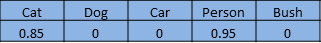
Neural networks for image recognition are usually trained to recognize a set of objects. Suppose we give each object an index from one to n. The classification network answers the question “What objects in this image?” Returning an array from zero to n-1, where each array record has a value from zero to one. Zero means that the object is not in the image. A nonzero value means that it can be there with increasing probability when the value approaches unity. Here is a cat and a man in an array of 5 elements:
A segmented network segments image pixels of areas that are occupied by objects from our list. She answers the question by returning an array with a record corresponding to each pixel in the image. Each record has a value of zero if it is a background pixel, or a value from one to n for n different objects that it can recognize. This fictional example may be the foot of a person:

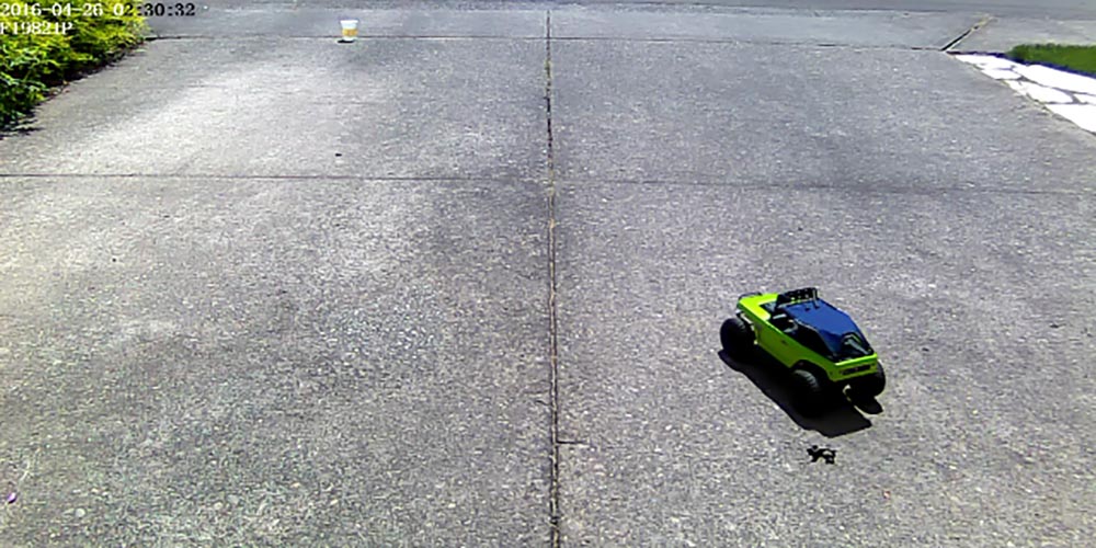
This project is part of a larger project aimed at controlling a radio-controlled car using a computer. The idea is to use a neural network to determine the position (global three-dimensional position and orientation) of a car for transmitting navigation commands to it. The camera is fixed, and the lawn is mostly flat. I can use the trigger a bit to change the 3d position so that the neural network can find the screen pixels and orientation. The cat’s role in all of this is the “intended purpose”.
I started by thinking primarily about the car, because I did not know how it would turn out, assuming that recognizing a cat with a pre-trained network would be trivial. After a lot of work, which I will not describe in detail in this article, I decided that you can determine the orientation of the car with a fairly high degree of reliability. Here is a training shot at an angle of 292.5 degrees:
Most of this work has been done with the classification network, the Caffe bvlc_reference_caffenet model. Therefore, I decided to let the segmentation network task determine the position of the machine on the screen.
The first network I used is Faster R-CNN [1]. It returns bounding boxes for objects in the image, not pixels. But the network on Jetson was too slow for this application. The idea of a bounding box was very attractive, so I also looked at the driving-oriented network [2]. She was also too slow. FCN [3] was the fastest segmentation network I tried. “FCN” means “Fully convolutional network”, fully convolutional network, since it no longer requires any specific image size to be input and consists only of convolutions / poolings. Switching only to convolutional layers leads to significant acceleration, classifying my images by about 1/3 second on Jetson. FCN includes a good set of Python scripts for training and easy deployment. Python scripts resize the network to fit any size of the incoming image, making it easy to process the main image. I had a winner!
The FCN GitHub release has several options. First I tried voc-fcn32s. It worked perfectly. Voc-fcn32s was pre-trained in 20 standard voc-classes. Since this is too simple, I tried pascalcontext-fcn32s. He was trained in 59 classes, including grass and trees, so I thought it should be better. But it turned out that not always - the output images had much more sets of pixels, and the segmentation of cats and people superimposed on grass and bushes was not so accurate. Segmentation from siftflow was even more complex, so I quickly returned to voc options.
Choosing voc networks still means three things to consider: voc-fcn32s, voc-fcn16s and voc-fcn8s. They differ in the “step” of output segmentation. Step 32 is the main step of the network: the 640x360 image is reduced to a 20x11 network by the time the convolutional layers are complete. This crude segmentation then “deconvolves” back to 640x360, as described in [3]. Step 16 and step 8 are achieved by adding more logic to the network for better segmentation. I didn’t even try - 32-segment segmentation is the first one I tried and it came up, and I stuck to it because segmentation looks good enough for this project, and training, as described, looks more complicated for the other two networks.
Training
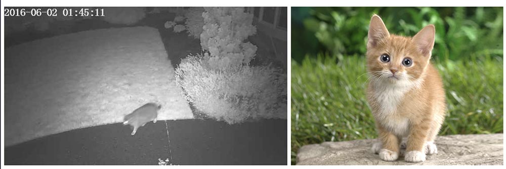
The first thing I noticed when I turned on and started the system was that only about 30% of the cats were recognized by the network. I found two reasons for this. Firstly, cats often come at night, so the camera sees them in infrared light. This can be easily fixed - just add some segmented infrared images of cats for training. The second problem that I discovered after reviewing several hundred photographs of cats from the training kit is that many of the photographs belong to the “look at my cute cat” variety. These are frontal images of a cat at the level of a cat's eye. Either the cat lies on its back or lies on its owner’s lap. They don't look like cats roaming around my yard. Again, it can be easily fixed with some segmented daytime images.
How to segment an object in a training image? My approach is to subtract the background image and then process the foreground pixels to indicate to track the object. In practice, this works pretty well, because in my archive from the camera there is usually an image that was taken a few seconds before the segmented image. But there are artifacts that need to be cleaned, and segmentation often needs to be clarified, so I wrote a rough preparation utility for editing image segments, src / extract_fg.cpp. See the note at the top of the source file for use. It is a little clumsy and has small verification errors and needs some refinement, but it works well enough for the task.
Now that we have some images for training, let's see how to do it. I cloned voc-fcn32s to the rgb_voc_fcn32s directory. All file names will refer to this directory until the end of this lesson.
$ cp -r voc-fcn32s rgb_voc_fcn32s
Code on my github, including sample training file in data / rgb_voc. The main changes are indicated below.
Training File Format
The distributed data layer expects hard-coded images and segmentation directories. The training file has one line per file; then the data layer gets the names of the image files and segments, adding hard-coded directory names. This did not work for me because I have several classes of training data. My training data has a set of lines, each of which contains an image and segmentation for that image.
$ head data/rgb_voc/train.txt /caffe/drive_rc/images/negs/MDAlarm_20160620-083644.jpg /caffe/drive_rc/images/empty_seg.png /caffe/drive_rc/images/yardp.fg/0128.jpg /caffe/drive_rc/images/yardp.seg/0128.png /caffe/drive_rc/images/negs/MDAlarm_20160619-174354.jpg /caffe/drive_rc/images/empty_seg.png /caffe/drive_rc/images/yardp.fg/0025.jpg /caffe/drive_rc/images/yardp.seg/0025.png /caffe/drive_rc/images/yardp.fg/0074.jpg /caffe/drive_rc/images/yardp.seg/0074.png /caffe/drive_rc/images/yard.fg/0048.jpg /caffe/drive_rc/images/yard.seg/0048.png /caffe/drive_rc/images/yard.fg/0226.jpg /caffe/drive_rc/images/yard.seg/0226.png
I replaced voc_layers.py with rgb_voc_layers.py, which understands the new scheme:
--- voc_layers.py 2016-05-20 10:04:35.426326765 -0700 +++ rgb_voc_layers.py 2016-05-31 08:59:29.680669202 -0700 ... - # load indices for images and labels - split_f = '{}/ImageSets/Segmentation/{}.txt'.format(self.voc_dir, - self.split) - self.indices = open(split_f, 'r').read().splitlines() + # load lines for images and labels + self.lines = open(self.input_file, 'r').read().splitlines()
And modified train.prototxt to use my rgb_voc_layers code. Note that the arguments are also different.
--- voc-fcn32s/train.prototxt 2016-05-03 09:32:05.276438269 -0700 +++ rgb_voc_fcn32s/train.prototxt 2016-05-27 15:47:36.496258195 -0700 @@ -4,9 +4,9 @@ top: "data" top: "label" python_param { - module: "layers" - layer: "SBDDSegDataLayer" - param_str: "{\'sbdd_dir\': \'../../data/sbdd/dataset\', \'seed\': 1337, \'split\': \'train\', \'mean\': (104.00699, 116.66877, 122.67892)}" + module: "rgb_voc_layers" + layer: "rgbDataLayer" + param_str: "{\'input_file\': \'data/rgb_voc/train.txt\', \'seed\': 1337, \'split\': \'train\', \'mean\': (104.00699, 1
Almost the same change in val.prototxt:
--- voc-fcn32s/val.prototxt 2016-05-03 09:32:05.276438269 -0700 +++ rgb_voc_fcn32s/val.prototxt 2016-05-27 15:47:44.092258203 -0700 @@ -4,9 +4,9 @@ top: "data" top: "label" python_param { - module: "layers" - layer: "VOCSegDataLayer" - param_str: "{\'voc_dir\': \'../../data/pascal/VOC2011\', \'seed\': 1337, \'split\': \'seg11valid\', \'mean\': (104.00699, 116.66877, 122.67892)}" + module: "rgb_voc_layers" + layer: "rgbDataLayer" + param_str: "{\'input_file\': \'data/rgb_voc/test.txt\', \'seed\': 1337, \'split\': \'seg11valid\', \'mean\': (104.00699, 116.66877, 122.67892)}"
Solver.py
Run solve.py to start your workout:
$ python rgb_voc_fcn32s / solve.py
It modifies some of the normal mechanisms of Caffe. In particular, the number of iterations is set at the bottom of the file. In this particular setup, the iteration is a single image because the network size changes for each image and the images are skipped one at a time.
One of the great things about working with Nvidia is that really great equipment is available. I have a Titan built into a workstation, and my management did not mind letting me use it for something as dubious as this project. My last training run was 4,000 iterations, which took a little over two hours on Titan.
I learned a few things
- A handful of images (less than 50) were enough to train the network to recognize night intruders.
- Night shots taught the network to think that the shadows on the footpath are cats.
- Negative shots, that is, images without segmented pixels, help combat the shadow problem.
- It’s easy to retrain the network using a stationary camera so that everything that is different is classified as something random.
- Cats and humans, superimposed on random backgrounds, help with problems that arise during overtraining.
As you can see, the process is iterative.
Recommendations
[1] Faster R-CNN: Towards Real-Time Object Detection with Region Proposal Networks Shaoqing Ren, Kaiming He, Ross Girshick, Jian Sun abs / 1506.01497v3 .
[2] An Empirical Evaluation of Deep Learning on Highway Driving Brody Huval, Tao Wang, Sameep Tandon, Jeff Kiske, Will Song, Joel Pazhayampallil, Mykhaylo Andriluka, Pranav Rajpurkar, Toki Migimatsu, Royce Cheng-Yue, Fernando Cojuj Mujica Andrew Y. Ng arXiv: 1504.01716v3 , github.com/brodyh/caffe.git .
[3] Fully Convolutional Networks for Semantic Segmentation Jonathan Long, Evan Shelhamer, Trevor Darrell arXiv: 1411.4038v2 , github.com/shelhamer/fcn.berkeleyvision.org.git .
conclusions
In order to teach the neural network to recognize night cats, it was necessary to add the necessary data, accumulating them. After this, the last step was taken - the system is connected to the valve that starts the sprayer. The idea is that as soon as the cat enters the lawn and wants to adapt, it starts to water. The cat dumps. The task is thus solved, the wife is happy, and all this strange miracle is a neural network that teaches to recognize cats, finds out that the Internet does not have enough source images for training and which has learned this, became the only neural network in the world that can recognize night cats.
It is worth noting that all this was done by a person who is not a hyperprogrammer who worked in Yandex or Google all his life and with the help of hardware, quite cheap, compact and simple.
A bit of advertising :)
Thank you for staying with us. Do you like our articles? Want to see more interesting materials? Support us by placing an order or recommending it to your friends, a 30% discount for Habr users on a unique analog entry-level server that we invented for you: The whole truth about VPS (KVM) E5-2650 v4 (6 Cores) 10GB DDR4 240GB SSD 1Gbps from $ 20 or how to divide the server? (options are available with RAID1 and RAID10, up to 24 cores and up to 40GB DDR4).
Dell R730xd 2 times cheaper? Only we have 2 x Intel TetraDeca-Core Xeon 2x E5-2697v3 2.6GHz 14C 64GB DDR4 4x960GB SSD 1Gbps 100 TV from $ 199 in the Netherlands! Dell R420 - 2x E5-2430 2.2Ghz 6C 128GB DDR3 2x960GB SSD 1Gbps 100TB - from $ 99! Read about How to Build Infrastructure Bldg. class c using Dell R730xd E5-2650 v4 servers costing 9,000 euros for a penny?