Stochastic gradient descent (SGD) for the logarithmic loss function (LogLoss) in a binary classification problem

The previous part (about linear regression, gradient descent and how it all works) - habr.com/en/post/471458



In this article, I will show the solution to the classification problem first, as they say, “pens”, without third-party libraries for SGD, LogLoss, and calculating gradients, and then using the PyTorch library.



Task: for two categorical features describing yellowness and symmetry, determine which class (apple or pear) the object belongs to (teach the model to classify objects).



To get started, upload our dataset:

import pandas as pd data = pd.read_csv("https://raw.githubusercontent.com/DLSchool/dlschool_old/master/materials/homeworks/hw04/data/apples_pears.csv") data.head(10)
      
      

        
        
        
      

    
        
        
        
      
      

        
        
        
      

    
     

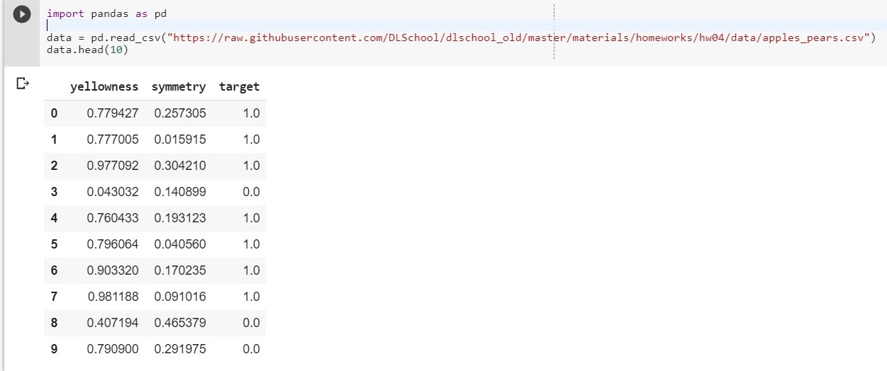
Let: x1 - yellowness, x2 - symmetry, y = targer



We compose the function y = w1 * x1 + w2 * x2 + w0

(w0 will be considered the bias (eng. - bias))



Now our task is reduced to finding weights w1, w2 and w0, which most accurately describe the dependence of y on x1 and x2.



We use the logarithmic loss function:







The left parameter of the function is the prediction with the current weights w1, w2, w0



The right parameter of the function is the correct value (class is 0 or 1)



σ (x) is the sigmoid activation function of x



log (x) - the natural logarithm of x



It is clear that the smaller the value of the loss function, the better we have chosen the weights w1, w2, w0. To do this, choose a stochastic gradient descent .



I note that the formula for LogLoss will take a different look in view of the fact that in SGD we select one element and not an entire selection (or a subsample, as is the case with mini-batch gradient descent):





Solution progress:



The initial weights w1, w2, w0 are given random values



We take a certain i-th object of our dataset (for example, random), calculate LogLoss for it (with our w1, w2 and w0, to which we initially assigned random values), then we calculate the partial derivatives for each of the weights w1, w2 and w0, then update each of the weights.



A little preparation:

 import pandas as pd import numpy as np X = data.iloc[:,:2].values #  - y = data['target'].values.reshape((-1, 1)) #  (    ) x1 = X[:, 0] x2 = X[:, 1] def sigmoid(x): return 1 / (1 + np.exp(-x))
      
      

        
        
        
      

    
        
        
        
      
      

        
        
        
      

    
     

Implementation:

 import random np.random.seed(62) w1 = np.random.randn(1) w2 = np.random.randn(1) w0 = np.random.randn(1) print(w1, w2, w0) # form range 0..999 idx = np.arange(1000) # random shuffling np.random.shuffle(idx) x1, x2, y = x1[idx], x2[idx], y[idx] # learning rate lr = 0.001 # number of epochs n_epochs = 10000 for epoch in range(n_epochs): i = random.randint(0, 999) yhat = w1 * x1[i] + w2 * x2[i] + w0 w1_grad = -((y[i] - sigmoid(yhat)) * x1[i]) w2_grad = -((y[i] - sigmoid(yhat)) * x2[i]) w0_grad = -(y[i] - sigmoid(yhat)) w1 -= lr * w1_grad w2 -= lr * w2_grad w0 -= lr * w0_grad print(w1, w2, w0)
      
      

        
        
        
      

    
        
        
        
      
      

        
        
        
      

    
     

[0.49671415] [-0.1382643] [0.64768854]

[0.87991625] [-1.14098372] [0.22355905]



* _grad is the derivative of the corresponding weight. I will write the general formula:







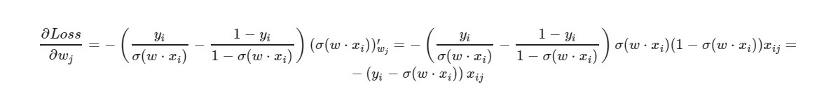
For the free term w0 - the factor x is omitted (taken equal to one).



According to the final formula of the derivative, we can see that we do not need to explicitly calculate the loss function (we only need partial derivatives).



Let's check on how many objects from the training set our model gives the correct answers, and on how many - the wrong ones.

 i = 0 correct = 0 incorrect = 0 for item in y: if(np.around(x1[i] * w1 + x2[i] * w2 + w0) == item): correct += 1 else: incorrect += 1 i = i + 1 print(correct, incorrect)
      
      

        
        
        
      

    
        
        
        
      
      

        
        
        
      

    
     

925 75



np.around (x) - rounds the value of x. For us: if x> 0.5, then the value is 1. If x ≤ 0.5, then the value is 0.



And what will we do if the number of features of the object is 5? 10? one hundred? And we will have the appropriate amount of weights (plus one for bias). It is clear that manually working with each weight, calculating gradients for it is inconvenient.



We will use the popular PyTorch library.



PyTorch = NumPy + CUDA + Autograd (automatic calculation of gradients)



PyTorch implementation:

 import torch import numpy as np from torch.nn import Linear, Sigmoid def make_train_step(model, loss_fn, optimizer): def train_step(x, y): model.train() yhat = model(x) loss = loss_fn(yhat, y) loss.backward() optimizer.step() optimizer.zero_grad() return loss.item() return train_step X = torch.FloatTensor(data.iloc[:,:2].values) y = torch.FloatTensor(data['target'].values.reshape((-1, 1))) from torch import optim, nn neuron = torch.nn.Sequential( Linear(2, out_features=1), Sigmoid() ) print(neuron.state_dict()) lr = 0.1 n_epochs = 10000 loss_fn = nn.MSELoss(reduction="mean") optimizer = optim.SGD(neuron.parameters(), lr=lr) train_step = make_train_step(neuron, loss_fn, optimizer) for epoch in range(n_epochs): loss = train_step(X, y) print(neuron.state_dict()) print(loss)
      
      

        
        
        
      

    
        
        
        
      
      

        
        
        
      

    
     

OrderedDict ([('0.weight', tensor ([[- 0.4148, -0.5838]])), ('0.bias', tensor ([0.5448])]])

OrderedDict ([('0.weight', tensor ([[5.4915, -8.2156]])), ('0.bias', tensor ([- 1.1130])]])

0.03930133953690529



Fairly good loss on the test sample.



Here, MSELoss is selected as a loss function.



More on Linear



In short: we give 2 parameters to the input (our x1 and x2 as in the previous example) and we get one parameter (y) to the output, which, in turn, is fed to the input of the activation function. And then they are already calculated: the value of the error function, gradients. At the end - weights are updated.



Materials used in the article