The heading "Read articles for you." January - June 2019

Hello, Habr! We continue to publish reviews of scientific articles from members of the Open Data Science community from the channel #article_essense. If you want to receive them before everyone else - join the community !

Articles for today:

1. Neural Ordinary Differential Equations (University of Toronto, 2018)
2. Semi-Unsupervised Learning with Deep Generative Models: Clustering and Classifying using Ultra-Sparse Labels (University of Oxford, The Alan Turing Institute, London, 2019)
3. Uncovering and Mitigating Algorithmic Bias through Learned Latent Structure (Massachusetts Institute of Technology, Harvard University, 2019)
4. Deep reinforcement learning from human preferences (OpenAI, DeepMind, 2017)
5. Exploring Randomly Wired Neural Networks for Image Recognition (Facebook AI Research, 2019)
6. Photofeeler-D3: A Neural Network with Voter Modeling for Dating Photo Rating (Photofeeler Inc., 2019)
7. MixMatch: A Holistic Approach to Semi-Supervised Learning (Google Reasearch, 2019)
8. Divide and Conquer the Embedding Space for Metric Learning (Heidelberg University, 2019)

1. Neural Ordinary Differential Equations

Authors of the article: Ricky TQ Chen, Yulia Rubanova, Jesse Bettencourt, David Duvenaud (University of Toronto, 2018)

→ Original article

Review author: George Ignatov (in slack a2dy2n7okhtp)

NIPS Best Paper Award

The authors of the article noted that ResNet-like networks are very similar to the Euler method for solving differential equations. If so, then why not immediately bring the idea to the maximum: imagine a neural network in the form of a differential equation and get

• A network with an arbitrary number of layers, which can be changed at any time during training and inference. More layers -> more precision and smoother conversions (and vice versa).
• A much smaller number of parameters, therefore, lower memory costs.

NODE through analogies:

1. $$$h_n = f_n (h_ {n-1}, W) + h_ {n-1}$ - this is how the definition of output from layer n in a resnet-like network looks like, W - parameters.
2. $$$h_n = f (h_ {n-1}, t = n, W) + h_ {n-1}$ - this would look like a NODE-like network, provided that n is a discrete quantity.
3. $$$h_n \ sim a f (t_n) + h_ {n-1}$ , $$$f (t) = dh (t) / dt$ - Euler's method.
4. $$$dh (t) / dt = f (h (t), t, W)$ - ta-da! ODE-powered neural network.

We solve it with any black-box ODEsolver, throw the gradients using the adjoint sensitivity method (Pontryagin et al., 1962). Due to its complete differentiability, NODE can be combined with conventional neural networks. The authors posted the code on pytorch.

The article discusses 3 applications:

1. Comparison with ResNet-like architecture (on MNIST). NODE works almost no worse, while using 3 times fewer parameters.
2. Overriding normalized flows through NODE - Continous Normalized Flows (synthetic dataset). The new model reduces computational overhead from O (n_hidden_units ^ 3) to linear.
3. Modeling of temporary events with irregular observations (synthetic dataset). A dataset of spiral trajectories was generated from which randomly sampled points sprinkled with: salt: Gaussian noise for plausibility. It tested the usual RNN and NODE, and the second again proved to be better.

In small print:

• Minibatch training causes some kind of computational overhead, but the authors argue that in practice this is almost invisible.
• Two new hyperparameters appear: network depth and error tolerance when solving ODE.
• For the ODE solution to remain unique, the network must have finite weights and use Lipshitz nonlinearities, such as tanh or relu.

Link to a more detailed overview on habr.

2. Semi-Unsupervised Learning with Deep Generative Models: Clustering and Classifying using Ultra-Sparse Labels

Article Authors: Matthew Willetts, Stephen Roberts and Christopher Holmes

(University of Oxford, The Alan Turing Institute, London, 2019)

→ Original article

Review author: Alex Chiron (in sliron shiron8bit)

The authors consider a semi-unsupervised case for the classification problem, when in the data markup due to selection bias some of the classes present were not labeled at all, and not so many were labeled according to known data classes. This creates additional problems, since most models usually work either in semi-supervised / supervised mode (classification) or in unsupervised mode (clustering), and in this case we need to consider both options. Moreover, the use of semi-supervised algorithms can lead to the fact that unallocated data will be assigned according to some metric of proximity to incorrect classes. A hypothetical example of such data is a set of tumor scans. We took part of the data and marked all the types of tumors present on this part, but it turned out that other types of tumors were also present in the remaining data, and the variability of the known species in the markup was not fully reflected.

The authors were inspired by deep generative models (the simplest example of such a model with a single layer depth of hidden variables is a variational auto-encoder, aka VAE): in previous works, such models successfully coped with both the semi-supervised case (M2, ADGM) and clustering ( VaDE, GM-VAE).

Why not solve 2 problems at the same time (semi-supervised learning on rarely marked up classes and unsupervised on unplaced classes), keeping the space of learned latent variables common and combining ideas from the above models? It is this idea that underlies the GM-DGM / AGM-DGM models proposed in the article.

Consider the M2 model in a semi-supervised case. It is called so, because under M1 the creator meant sequential training of VAE and some classifier (svm) for the resulting latent representations of z, but M2 is already obtained from VAE by adding to the layer of hidden variables the variable y, which is responsible for the sometimes observed class.

$$$p _ {\ theta} (x, y, z) = p _ {\ theta} (x | y, z) p (y) p (z)$ , $$$q _ {\ pi} (z, y | x) = q _ {\ pi} (z | y, x) q _ {\ pi} (y | x)$

Where $$$q _ {\ phi} (y | x) = Cat (\ pi _ {\ phi} (x))$ , $$$q _ {\ phi} (z | x, y) = N (z | \ mu _ {\ phi} (x, y), \ Sigma _ {\ phi} (x, y))$

Here q is an encoder, p is a decoder, part $$$q _ {\ phi} (y | x)$ - directly trained classifier.

For the unsupervised / semi-unsupervised case, M2 does not work - posterior collapse occurs, the classification part q_phi (y | x) collapses to the a priori distribution p (y). The author of GM-VAE in his article also showed the inoperability of M2 in practice and noted that often when implementing M2 the first layer of the h1 decoder is very similar to a mixture of Gaussians.

Based on this observation, GM-VAE uses an explicit layer of hidden variables for clustering a Gaussian mixture for clustering, which is also repeated by the authors of the article under review. Thus, the GM-DGM model, which allows successful operation in semi-unsupervised mode, is a modification VAE using a mixture of Gaussian in a hidden layer depending on a variable of class y, with the above function of two terms for counting and maximizing ELBO.

The authors of the article conducted an experiment on a semi-unsupervised version of Fashion-MNIST: they removed the labels of the first 5 classes, the remaining 5 classes left 5% of the labels, while they received a total accuracy of 77.2% against 53% for M2. The possibility of using the model for clustering was also shown (which is not surprising, because it is almost GM-VAE).

3. Uncovering and Mitigating Algorithmic Bias through Learned Latent Structure

Authors: Alexander Amini, Ava Soleimany, Wilko Schwarting, Sangeeta N. Bhatia, Daniela Rus (Massachusetts Institute of Technology, Harvard University, 2019)

→ Original article

Review author: Alex Chiron (in sliron shiron8bit)

Recently, more and more often in the media you can find news that touches on the topic of bias in data, especially regarding algorithms related to individuals - with the growth of their applicability, the risk of a strong negative impact on those categories and groups of people that are insufficient (or excessive) presented in dataset. One of the latest examples is a study that showed less accuracy in detecting pedestrians with dark skin color (in the context of object detection on standard BDD100K and MSCOCO datasets, link ). Basic approaches to eliminating biases:

1. Class balancing using resampling (requires a priori understanding of the hidden data structure).
2. Generation of unbiased data (for example, the use of GAN to generate individuals with a wide variety of skin tones ).
3. Clustering and subsequent resampling.
4. You can still wait until the IBM Diversity in Faces dataset is brought to academictorrents.

The authors of the article offer a modification of VAE and sampling taking into account the distribution of the latent variable z, which allows reducing the influence of bias in the data at the training stage.

So, the main ideas behind DB-VAE are:

• Consider a classification problem in which we have a training dataset {(x, y)}, x are m-dimensional features, y are d-dimensional labels, and our task is to approximate the mapping X-> Y.
• Let's take VAE, but in addition to the vector z of hidden variables z of dimension 2k we will force the encoder (I recall 2 here because we are dealing with averages and variances) to also learn a vector of dimension d, which is responsible for the aforementioned labels. In this case, the decoder accepts only the vector z as input. Thus, we get a semblance of semi-supervised learning, where part of the model is learned to reconstruct input, and part is to solve a specific problem (classification).
• We control the training of the model due to the combined loss, combining the standard loss for VAE (reconstruction + KL divergence) and the loss for an auxiliary problem (for example, cross-entropy for the binary classification problem).
• Particular attention is paid to the fact that you need to control training on data that you do not want to debiasing (that is, do not do backprop on them from the decoder).

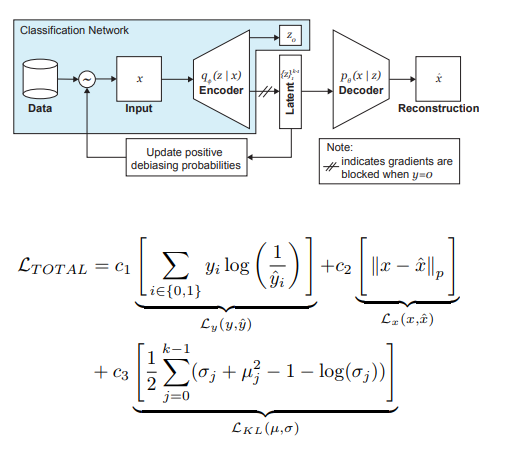
The most important role in eliminating the pain of blacks is played by adaptive sampling at the training stage. We want to choose rare (from the point of view of some hidden, not explicitly allocated factors) samples, so we turn to the histograms for each dimension of the space of hidden variables z, the product of which can approximate the distribution Q (z | X) of data over the entire space Z. When forming a new batch, we will take into account the 'inverse' to Q (z | X) distribution W (z (x) | X), which determines the probability of choosing an example in the batch (alpha is a hyper parameter that determines the degree of debiasing), updating Q (z | X) in every era. As you can see, debiasing is not selected in advance, but is done based on the learned latent variables.

As an experiment, the authors solved the problem of binary classification (finding the face in the photo). For training, we collected a dataset, which consisted of 200 thousand people with CelebA and 200 thousand non-people with Imagenet, resized images to 64x64. As mentioned earlier, during training, backpropagation from the decoder for photos without faces was blocked (y = 0). After training, they were validated on the Pilot Parliaments Benchmark (PPB) (1270 photos of people from the parliaments of South Africa, Rwanda, Senegal, Sweden, Finland, Iceland): for all alpha> 0, the detection accuracy in the categories dark male, dark female, light female increased compared to option without debiasing.

4. Deep reinforcement learning from human preferences

Authors: Paul Christiano, Jan Leike, Tom B. Brown, Miljan Martic, Shane Legg, Dario Amodei (OpenAI, DeepMind, 2017)

→ Original article

Review author: Dmitry Nikulin (in dniku slack)

This article is about how to implement the old idea in the context of deep reinforcement learning (RL). Idea: let's ask a person to evaluate the behavior of the agent, and based on this we will learn the reward function. The problem is that deep RL is very voracious, and human time is expensive. The article provides a set of hacks that allow you to reduce human hours to reasonable values.

Reward function is a function on pairs (observation, action). It is set by averaging the prediction of an ensemble of neural networks. The RL algorithms used (in the article A2C for Atari and TRPO for Mujoco) believe that this average is a true reward, and are trained on it. Thus, the article focuses on the issue of training this ensemble.

The ensemble is trained on human evaluations. Each rating is structured as follows. A person is shown two videos of an agent 1-2 seconds long. He can rate such a pair in 4 ways: left is better / right is better / too similar / uncomparable. If a person said "uncomparable", then such an assessment is thrown away. Otherwise, the triple (σ¹, σ², μ) is remembered, where σⁱ is the trajectory of the agent in the corresponding video (i.e., the list of pairs (obs, act)), and μ is the pair (1, 0), (0, 1 ) or (½, ½). Further, it is believed that the prediction of the reward for the trajectory is equal to the sum of the predictions for each pair (obs, act). Finally, we simply optimize softmax_cross_entropy_with_logits.

It is believed that a person with a 10% probability selects a random answer, and this is taken into account when constructing a training sample. Section 2.2.3 of the article gives a few more tricks and writes out all the formulas.

Pairs of clips for demonstration to a person are selected as follows: a large number of clips are sampled, the dispersion of the ensemble is considered on them, and random pairs of clips with high dispersion are shown to people. The authors say that I would like to choose according to the value of information, but this is future work.

The authors run tests on Atari and Mujoco, with real human ratings (hired contractors) and synthetic (ratings are generated according to the true reward function), and at the same time they are compared with the usual RL. With approximately equal numbers of ratings, synthetic and real tests work similarly. Moreover, surprisingly, regular RL (which sees the true reward function) does not necessarily work better.

Finally, in addition to trying to train the agent to get a lot of reward in the usual sense, the article also gives examples of two other tasks: the Hopper in Mujoco does a backflip, and the machine in Atari Enduro does not overtake other cars, but travels parallel to them. It turned out to solve both problems.

In conclusion: the example describes an attempt to reproduce this article. The attempt was successful, but it took 8 months of work in free time and 220 hours of pure time, of which half went to debug the simplest version.

5. Exploring Randomly Wired Neural Networks for Image Recognition

Authors: Saining Xie, Alexander Kirillov, Ross Girshick, Kaiming He (Facebook AI Research, 2019)

→ Original article

Review author: Egor Panfilov (in slack tutk1ja)

Introduction:

The paper addresses the issue of generation of neural network architecture. Currently, many architectural tricks are known (LSTM, Inception, ResNet, DenseNet), which can improve the quality of many tasks, but they also introduce a certain strong architectural prior into the model. Instead of the mentioned solutions, google is pushing ahead with its neural architecture search (NAS), where the architecture search for a specific task is carried out from predefined modules via RL - NASNet, AmoebaNet.

The authors argue that both approaches where the design is determined by man and NAS introduce too strict prior to the architecture. In an attempt to reduce it, they attempt to use the parametric generative approach of the neural network, where the wiring (connection) of elements is carried out randomly. It turns out that random wiring approaches have been explored since the 1940s by such scientists as A. Turing, M. Minsky, F. Rosenblatt. As another argument, the authors recall that in neuroscientific studies it was revealed that the structure of neuronal connections in organisms of one species is different (to a certain level of detail, of course). This is true for both worms and human babies. In general, the idea of ​​procedural generation of neural networks sounds interesting and promising, which is what the work is about.

Method:

Let's try to modularize the process of procedural generation of neural network architecture through a graph approach. The initial steps are as follows:

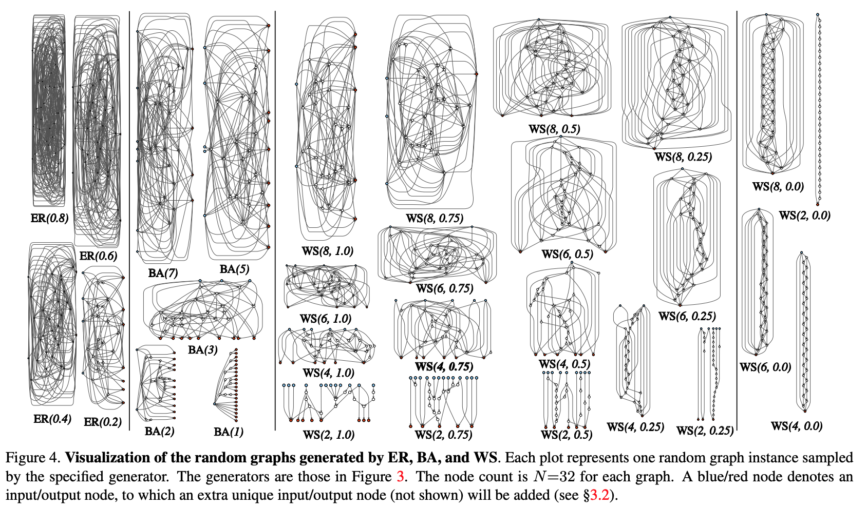
1. A stochastic graph is generated from a parametrized family. Classic methods are used: Erdos-Renyi (ER), Barabasi-Albert (BA), and Watts-Strogatz (WS).
2. The graph is converted to a neural network:
   
   
   • all edges of the graph are assumed to be directed carriers of data tensors;
   • for each vertex of the graph, the type of operation that it performs is determined: (I) aggregation by summing with the trained weights, (II) transformation - ReLU + convolution + BN, (III) distribution - transfer of the tensor along each output edge;
   • according to the results of the previous subclause, there can be several input and output vertices, but I want to have 1 entry point in the graph and 1 output point. Such nodes are created separately. The input one simply spreads a copy of the tensor to all the input vertices of the graph, the output one considers the unweighted average of all output vertices. As a result of steps 1 and 2, in fact, not a complete network is created, but only one of the modules (like conv_1, ... in popular convolutional encoders). In order to get the neural network completely:
3. Several modules are created and connected in series. To reduce the number of network parameters, transformations at all input vertices of the modules are performed with a stride of 2x2. The number of channels in the transition to the next module increases by 2 times. To conduct experiments on a specific task:
4. At the output of the network, a head is added for classification.

Results:

Testing of the method was carried out on the classification problem on ImageNet. The quality of the generated neural network turned out to be on par with SotA architectures, losing a bit to the recent Google's DeepBrain AmoebaNet: (with a comparable number of parameters).

We checked what would happen if we removed a random vertex / edge from the resulting graph. Metric - quality reduction depending on the adjacent number of output edges / input vertices, respectively. In general, the quality is falling, but not critical.

The authors also checked whether transfer learning works with this architecture. In the COCO detection task, the backbone Faster R-CNN with FPN was replaced with a generated and pre-trained network. The results showed that the quality of the model is not worse than that of ResNeXt-50 / -101. But even the fact that transfer learning is starting up is pretty entertaining.

6. Photofeeler-D3: A Neural Network with Voter Modeling for Dating Photo Rating

Authors of the article: Agastya Kalra and Ben Peterson (Photofeeler Inc., 2019)

→ Original article

Review author: Alex Chiron (in sliron shiron8bit)

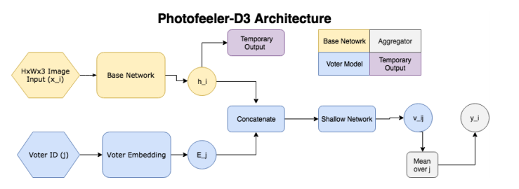
The authors propose Photofeeler-D3: a network architecture for evaluating photos from dating sites in 3 directions / traits - as far as a person seems smart, trustworthy and attractive (neglect the halo effect!). The task arose based on a survey by The Guardian, according to which 90% of people decide on a future date solely on the basis of evaluating photos of a potential satellite

So, the network consists of the following blocks:

1. The base network (the yellow part in the picture) - we get embedding from the pre-trained classification grid (GAP after convolutional layers), then we pass it through a fully connected layer with 10 outputs (and softmax) - we get a temporary output.
2. In the second block (the blue part, the voter model), one who voted for the image (voter) is selected, its embedding is taken, concatenated with temporary output from the base block, after which the resulting vector is fed to the input of a small fully connected network, at the output of which we obtain the distribution over 10 classes v_ij ((distribution over 10 intervals inside [0; 1]). A numerical estimate is obtained by the scalar product v_ij with the vector [0.05, 0.15, 0.25 ... 0.95].
3. We have a rating for the image and the individual voter, and averaging it over 200 arbitrary voters, we get the final rating.

Voting modeling means that we are not trying to predict a potentially noisy average estimate, we only predict the subjective opinion of a particular voter, which means that the number of votes on the image is not so much affected, and noise from images with a small number of votes is less. In literature, there is a similar Facial problem Beauty Prediction (FBP) with open SCUT-FBP and Hot-Or-Not datasets, however, the authors used data obtained directly from the Photofeeler website for training, where each user is evaluated using the above parameters THER users. At the same time, there is a lot of data: + 100k ratings arrive on the site every day, they took 1.2 million photos in total, of which a million men (200 thousand unique people) and 200 thousand women (50 thousand unique people). All photos with different aspect ratios, but no more than 600px. For testing, 10,000 photographs of men and 8,000 photographs of women were separated. It should be noted that the original grades on the site go from 0 to 3, but the final grade for training and testing was normalized and was reduced to the interval [0,1] by averaging over all those who voted with weights ( weights were determined based on the characteristics of a particular person's vote).

Important points when learning:

1. Hyperparameters (backbone for embedding, picture size, etc) were chosen when training on a smaller data set (20000 train, 3000 val, 2311 test), the best results are obtained for the xception architecture and 600x600 pictures.
2. First, the basic network is trained, the output of which (temporary output) is compared by KL divergence with the actual distribution of ratings for the photo (as I wrote a little earlier, we first normalize each rating, then build the distribution over 10 bins on the interval [0,1]).
3. For voter model training, a specific grade is converted to one-hot rounding to the nearest tenths.
4. Voter embers are also likely to learn, and the base model is frozen at stage 2.
5. Models for all three types of traits and 2 genders were trained separately, estimates of only the opposite sex were used. Results:
   
   
   • For both sexes, the model showed a correlation of ~ 80% with human ratings on their internal dataset, while at London Faces architecture showed a much higher correlation with people than prettyscale.com and hotness.ai (81 versus 53 and 52).
   • In the FBP problem on both datasets (SCUT-FBP and Hot-Or-Not), results close to SOTA were obtained.
   • Tests also show that the model behaves better than averaging over 10 people who vote.

7. MixMatch: A Holistic Approach to Semi-Supervised Learning

Authors: D. Berthelot, N. Carlini, IJ Goodfellow, N. Papernot, A. Oliver and Colin Raffel (Google Reasearch, 2019)

→ Original article

The author of the review: Sergey Chervontsev (in slack JanRocketMan)

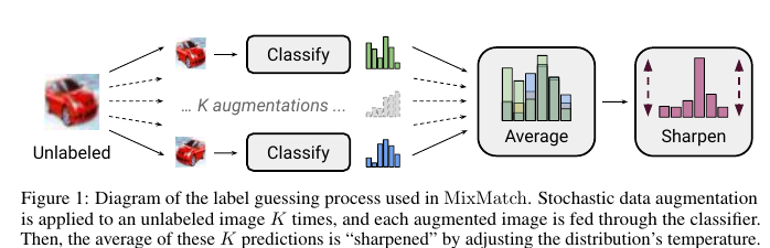
A mixture of MeanTeacher and Mixup for the new SOT in the Semi-Supervised Learning (SSL) task of classifying pictures. Let me remind you that the most working SSL now relies on consistency regularization. This means that in addition to the usual loss on the train (which is small and with which everything is overfitted) on unallocated data, we either use “noisy” marks, or do local perturbations and teach the model to produce the same predictions regardless of them. An example of the first approach is Mean Teacher ( where noisy labels are predictions of a model with EMA weights), an example of the second is Mixup (although it doesn’t ditch a bit). The authors offer something in between, plus a few hyperparameters to better control what is happening. It works like this:

1. We re-sample the unsupervised picture with different augmentations several times, and average the predictions.
   
   We get a “noisy” label p.
2. We “sharpen” the resulting class distribution so that it is closer to one-hot. The following conversion is proposed: $$$p_ {new} = p ^ {1 / T} / sum (p ^ {1 / T}, dim = 1)$ . By changing T, you can balance between the fact that the distribution is smeared, but the quality of the labels is good and the distribution is more like the true one (in shape), but the quality of the labels sags.
3. Everything mixes up with everything, randomly breaking up into pairs. Despite such minor changes, they are great brought to SVHN, STL and CIFAR10.

On CIFAR10 they have approximately 90% accuracy using only 250 tags. For comparison, the second in quality - VAT, gives only 60%. On SVHN, somewhere around 96% also have 250 marks, when VAT and Mean Teacher give closer to 90.

On STL10, 90% with 1k tags, put some CCGAN in comparison, which gives 80. In general, encouraging results showing that:

1. Bold models are good, even when there is little data (but the task is simple);
2. With straight arms and GridSearch, and simple approaches give significant profit;
   
   c. SSL can already get out of the SVHN sandbox and work with more complex datasets.

8. Divide and Conquer the Embedding Space for Metric Learning

: Artsiom Sanakoyeu, Vadim Tschernezki, Uta Buchler and Bjorn Ommer (Heidelberg University, 2019)

→

: ( Alexander Denisenko)

— , . , , – , , , ..

, :

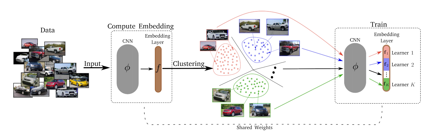
2. Divide.
   
   - k-means. . . Embedding layer K . – . d/K (d – ).
3. Conquer.
   
   Divide K K . , , , -, , . , T (Divide) .
4. – ( ). , .

: .

– Triplet Loss, Margin Loss, Proxy-NCA, ..

K 8 ( 128, 16- ).

T 1 10 , T=2.