Bond Portfolio Optimization Using ALGLIB
The article, due to the presence of a small amount of mathematics in it, may seem complicated to someone. But if you decide to start investing, then you need to be prepared for the fact that mathematics is often found in financial reality and is even more complicated.
The source code of the program and an example portfolio for optimization are posted on GitHub.
So, we have the task of forming an effective portfolio of bonds.
Part 1. Determination of the duration of the portfolio
From the point of view of minimizing non-systemic risks (for which the portfolio is diversified), the choice of securities was carried out by considering the parameters of a particular issue, issuer (if not limited to OFZ ), the behavior of the paper, etc. (approaches to such an analysis are quite individual for each investor and are not considered in this article).
Having selected several securities that are most preferable for investment, a natural question arises: how many pieces of bonds of each issue do you need to buy? This is the task of optimizing the portfolio so that the risks of the portfolio are minimal.
It is natural to consider duration as an optimized parameter. Thus, the task is to determine the weight of the securities in the portfolio, such that the duration of the portfolio would be minimal with some fixed portfolio yield. Here you need to make a few reservations:
- The duration of the bond portfolio is determined by its constituent securities. These durations are known (they are in the public domain). Portfolio duration is not equal to the maximum duration of the securities included in it (there is such a fallacy). The relationship between the durations of individual securities and the duration of the entire portfolio is not linear, i.e. is not equal to the weighted average duration of its constituent bonds (To verify this, it is enough to consider the duration formula (see (1) below) and try to calculate the weighted average duration of a conditional portfolio consisting, for example, of two papers. Substituting the formula for duration into such an expression of each paper, at the output, we get not a formula for the duration of the portfolio, but a kind of “nonsense”, with two discount rates and inconsistent cash flows as weights).
- Unlike duration, portfolio return depends on the returns of the instruments included in it linearly. Those. placing money in several instruments with a fixed income, we will get a return directly proportional to the volume of investments in each instrument (and this works for a complex rate, and not just for a simple one). Make sure this is even easier.
- The yield to maturity ( YTM ) is used as the bond yield rate. It is usually used to calculate duration. However, the yield to maturity of the entire portfolio here is rather arbitrary, since the maturity of all securities is different. When forming a portfolio, this feature must be taken into account in the sense that the portfolio should be reviewed, no less than the tools from which it is composed, go out of circulation.
So, the first task is the correct calculation of the duration of the portfolio itself. The immediate way to do this is to: determine all payments for the portfolio, calculate the yield to maturity, discount payments, multiply the received values by the terms of these payments and summarize. In order to do this, you need to combine the payment calendars of all instruments into a single payment calendar for the entire portfolio, compose an expression for calculating the yield to maturity, calculate it, discount it for each payment, multiply by its due date, add ... In general, a nightmare. Even for two papers, doing this is a very laborious task, not to mention regularly recalculating the portfolio in the future. This way does not suit us.
Therefore, it is necessary to look for an opportunity to determine the duration of the portfolio in another, faster way. An acceptable option would be one that allows you to determine the duration of the portfolio by known instrument durations. Studies of the duration formula showed that there is such a path and here I would like to give it in detail (if someone is not interested in the mathematical details of the calculations, you can safely skip a few paragraphs with the formulas and go straight to the example).
The duration of a debt instrument is defined as follows:
$$ display $$ \ begin {equation} D = \ frac {\ sum_ {i} PV_i \ cdot t_i} {\ sum_ {i} PV_i} ~~~~~~~~~~~~~ (1) \ end {equation} $$ display $$
Where:
- t i is the time moment of the i-th payment;
- $ inline $ \ begin {equation} PV_i = \ frac {CF_i} {(1 + r) ^ {t_i}} \ end {equation} $ inline $ - i-th discounted payment;
- CF i - i-th payment;
- r is the discount rate.
We introduce the discount coefficient k = (1 + r) and consider the amount of discounted payments P as a function of k :
$$ display $$ \ begin {equation} P (k) = \ sum_ {i} PV_i = \ sum_ {i} {\ frac {CF_i} {k ^ {t_i}}} ~~~~~~~~~ ~~~~ (2) \ end {equation} $$ display $$
Differentiating P with respect to k, we obtain
$$ display $$ \ begin {equation} P '(k) = - \ sum_ {i} {t_i \ frac {CF_i} {k ^ {t_i + 1}}} = - \ frac {1} {k} \ sum_ {i} {t_i \ frac {CF_i} {k ^ {t_i}}} ~~~~~~~~~~~~~ (3) \ end {equation} $$ display $$
Given the latter, the expression for the duration of the bond takes the form
$$ display $$ \ begin {equation} D = -k \ frac {P '(k)} {P (k)} ~~~~~~~~~~~~~ (4) \ end {equation} $$ display $$
At the same time, we recall that as a discount rate r in the case of a bond, yield to maturity (YTM) is used.
The resulting expression is valid for one bond, but we are interested in a portfolio of bonds. Let's move on to the definition of portfolio duration.
We introduce the following notation:
- P i - price of the i-th bond;
- z i - the number of securities of the i-th bond in the portfolio;
- k i - discount coefficient of the i-th bond in the portfolio;
- $ inline $ \ begin {equation} P_p = \ sum_ {i} {z_iP_i} \ end {equation} $ inline $ - portfolio price;
- $ inline $ \ begin {equation} w_i = \ frac {z_iP_i} {\ sum_ {i} z_iP_i} = \ frac {z_iP_i} {P_p} \ end {equation} $ inline $ - the weight of the i-th bond in the portfolio; obvious requirement $ inline $ \ begin {equation} \ sum_ {i} w_i = 1 \ end {equation} $ inline $ ;
- $ inline $ \ begin {equation} k_p = \ sum_ {i} w_ik_i \ end {equation} $ inline $ - portfolio discount coefficient;
Due to the linearity of differentiation, the following is true:
$$ display $$ \ begin {equation} P'_p (k) = \ left (\ sum_ {i} z_iP_i (k) \ right) '= \ sum_ {i} z_iP'_i (k) ~~~~~ ~~~~~~~~ (5) \ end {equation} $$ display $$
Thus, taking into account (4) and (5), the duration of the portfolio can be expressed as
$$ display $$ \ begin {equation} D_p = -k_p \ frac {P'_p} {P_p} = - \ sum_ {i} w_ik_i \ left (\ frac {\ sum_ {j} z_jP'_j} {\ sum_ {j} z_jP_j} \ right) ~~~~~~~~~~~~~~ (6) \ end {equation} $$ display $$
From (4) it follows unambiguously $ inline $ \ begin {equation} P'_j = - \ frac {D_jP_j} {k_j} \ end {equation} $ inline $ .
Substituting this expression in (6), we arrive at the following formula for portfolio duration:
$$ display $$ \ begin {equation} D_p = \ sum_ {i} w_ik_i \ left (\ frac {\ sum_ {j} \ frac {D_j} {k_j} z_jP_j} {\ sum_ {j} z_jP_j} \ right) = \ left (\ sum_ {i} w_ik_i \ right) \ left (\ sum_ {j} w_j \ frac {D_j} {k_j} \ right) ~~~~~~~~~~~~~ (7) \ end {equation} $$ display $$
In conditions when the duration and yield to maturity of each instrument are known (and we recall, we are in just such conditions), expression (7) is the desired formula for determining the duration of a portfolio based on the duration of its bonds. It only seems complicated in appearance, but in fact it is already ready for practical use with the help of the simplest functions of MS Excel, which we will now do with an example.
Example
To calculate the duration of the portfolio according to formula (7), we need the initial data, including the actual set of securities included in the portfolio, their durations and yield to maturity. As mentioned above, this information is publicly available, for example, on the website rusbonds.ru in the analysis of bonds section. Source data can be downloaded in Excel format.
As an example, consider a portfolio of securities consisting of 9 bonds. The original data table downloaded from rusbonds has the following form.
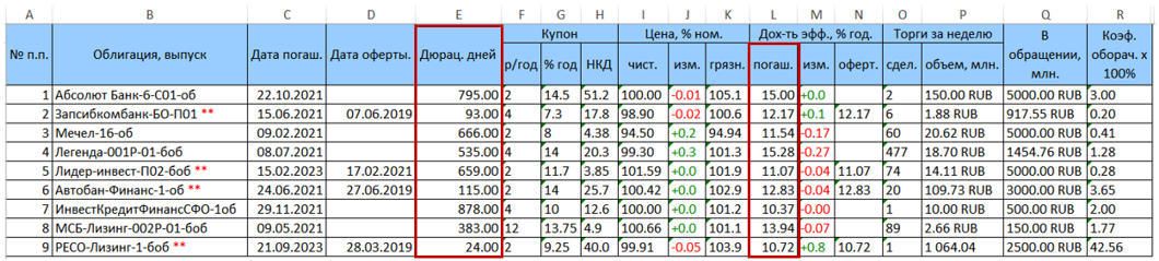
Two columns of interest to us with duration (column E) and yield to maturity (column L = YTM) are highlighted in red.
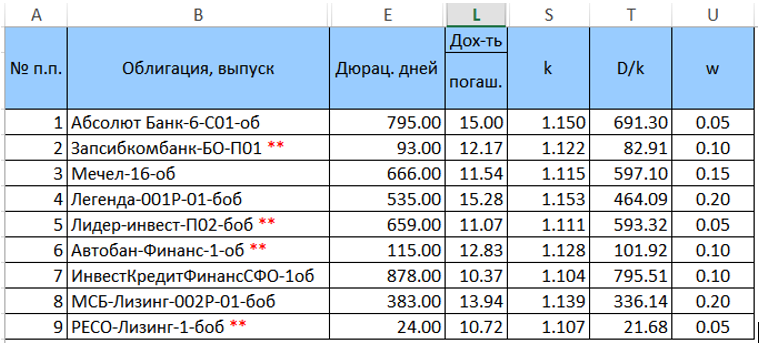
We set the weights w for bonds in this portfolio (so far in an arbitrary way, but so that their sum is equal to unity) and calculate k = (1 + YTM / 100) and D / k = (“column E” / k). The converted table (without extra columns) will look like
Next, we calculate the product $ inline $ \ begin {equation} w_j \ frac {D_j} {k_j} \ end {equation} $ inline $ and $ inline $ \ begin {equation} w_ik_i \ end {equation} $ inline $ and sum them up, and multiply the resulting amounts by one by the other. The result of this multiplication will be the desired duration for a given distribution of weights.
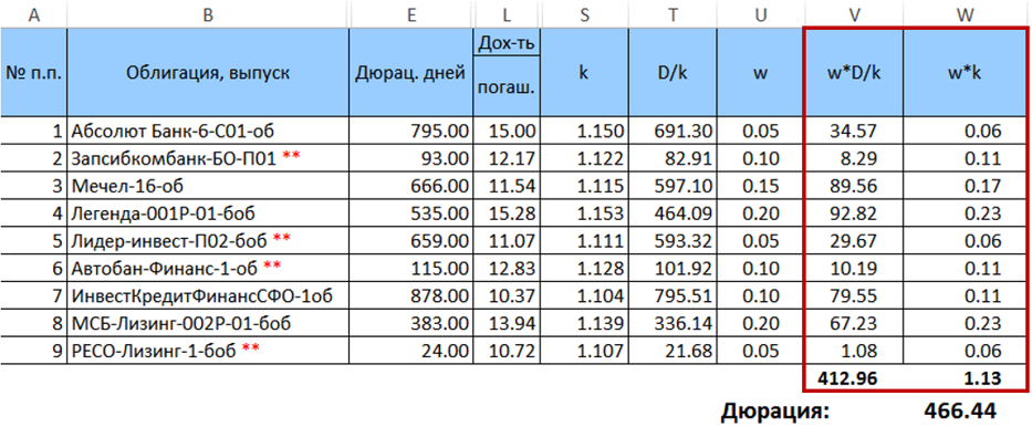
So, the desired duration of the portfolio is 466.44 days. It is important to note that in this particular case, the duration calculated by formula (7) is very slightly different from the weighted average duration calculated with the same weights (deviation <0.5 days). However, this difference increases with an increase in the spread of the weights. It will also increase with an increase in the spread of paper durations.
After we have obtained the formula for calculating the duration of the portfolio, the next step is to determine the weight of the securities so that at a given yield, the estimated duration of the portfolio would be minimal. We move on to the next part - portfolio optimization.
Part 2. Bond Portfolio Optimization
Expression (7) is a quadratic form, with the matrix
$$ display $$ \ begin {equation} A = \ left \ {k_i \ frac {D_j} {k_j} \ right \} = \ begin {pmatrix} D_1 & \ ldots & k_1 \ frac {D_n} {k_n} \ \ \ vdots & D_j & \ vdots \\ k_n \ frac {D_1} {k_1} & \ ldots & D_n \ end {pmatrix} \ end {equation} $$ display $$
Accordingly, in matrix form, the expression for the duration of the portfolio (7) can be written as follows:
$$ display $$ \ begin {equation} D_p = w ^ TAw ~~~~~~~~~~~~~ (8) \ end {equation} $$ display $$
where w is the column vector of the bond weights in the portfolio. As mentioned above, the sum of the elements of the vector w must be equal to unity. On the other hand, the expression $ inline $ k_p = \ sum_ {i} w_i k_i $ inline $ (which, in fact, is a simple scalar product ( w , k ) , where k is the vector of bond discount coefficients) should be equal to the target discount rate of the portfolio, and therefore the target portfolio return should be set.
Thus, the task of optimizing a bond portfolio is to minimize the quadratic function (8) with linear constraints.
The classical method of finding the conditional extremum of a function of several variables is the Lagrange multiplier method. However, this method is not applicable here, if only because the matrix A is degenerate by construction (but not only because of this; we omit the details of the analysis of the applicability of the Lagrange method here so as not to overload the article with excessive mathematical content).
The inability to apply an easy and affordable analytical method leads to the need to use numerical methods. The problem of optimizing a quadratic function is well known and has several long-developed efficient algorithms implemented in public libraries.
To solve this particular problem, the ALGLIB library and the quadratic optimization algorithms implemented in it, QP-Solvers , included in the minqp package, were used.
The quadratic optimization problem in general is as follows:
It is required to find an n-dimensional vector w minimizing the function
$$ display $$ \ begin {equation} F = \ frac {1} {2} w ^ T Qw + b ^ T w ~~~~~~~~~~~~~ (9) \ end {equation} $$ display $$
With given restrictions
1) l ≤ w ≤ u ;
2) Cw * d ;
where w, l, u, d, b are n-dimensional real-valued vectors, Q is the symmetric matrix of the quadratic part, and the sign * means any of the relations ≥ = ≤.
As can be seen from (8), the linear part b T w in our objective function is equal to zero. However, matrix A is not symmetric, which, however, does not prevent one from bringing it to a symmetrical form without changing the function itself. To do this, just put instead of A the expression $ inline $ \ begin {equation} \ frac {A ^ T + A} {2} \ end {equation} $ inline $ . Since formula (9) includes the coefficient $ inline $ \ frac {1} {2} $ inline $ then we as Q we can accept $ inline $ A ^ T + A $ inline $ .
The coordinates of the vectors l and u specify the boundaries of the desired vector and lie in the range [-1,1]. Since we do not assume short sales of bonds, the coordinates of the vectors in our case are all no less than 0. In the example program below, for simplicity, the vector l is assumed to be zero, and the coefficients of the vector u are all 0.3 . However, nothing prevents us from improving the program and making the constraint vectors more customizable.
Matrix C in our case will consist of two rows: 1) discount coefficients, which, when scalarly multiplied by weights (the same ( w , k )), should give the target rate of return on the portfolio; 2) a string consisting of units. It is needed to set limits $ inline $ \ sum_ {i} w_i = 1 $ inline $ .
Thus, the expression Cw * d for our task will look like this:
$$ display $$ \ begin {equation} \ left \ {\ begin {array} {ccc} ({\ bf w, k}) = k_p \\ \ sum_ {i} w_i = 1 \\ \ end {array} \ right. ~~~~~~~~~~~~~ (10) \ end {equation} $$ display $$
We now turn to the software implementation of the search for the optimal portfolio. The basis of the quadratic optimizer in ALGLIB is the object $ inline $ \ tt \ small minqpstate $ inline $
alglib::minqpstate state;
To initialize the optimizer, this object is passed to the minqpcreate function along with the task dimension parameter n
alglib::minqpcreate(n, state);
The next most important point is the choice of optimization algorithm (solver). The ALGLIB library for quadratic optimization offers three solvers:
- QP-BLEIC is the most universal algorithm designed to solve problems with not very large (up to 50 according to the recommendations of the documentation) number of linear constraints (of the form Cw * d ). At the same time, it can be effective on tasks of large dimension (as the documentation claims - up to n = 10000).
- QuickQP is a very efficient algorithm, especially when a convex function is optimized. However, unfortunately, it cannot work with linear constraints - only with boundary conditions (of the form l≤w≤u ).
- Dense-AUL - optimized for the case of very large dimensions and a large number of restrictions. But, according to the documentation, tasks of small dimension and the number of restrictions will be more efficiently solved using other algorithms.
Given the above characteristics, it is obvious that the QP-BLEIC solver is most suitable for our task.
In order to instruct the optimizer to use this algorithm, you must call the function $ inline $ \ tt \ small minqpsetalgobleic $ inline $ . The object itself and the stopping criteria are passed to this function, which we will not dwell on in more detail: the program considered here uses the default values. The function call is as follows:
alglib::minqpsetalgobleic(state, 0.0, 0.0, 0.0, 0);
Further initialization of the solver includes:
- The transfer of the matrix of the quadratic part Q - $ inline $ \ tt \ small alglib :: minqpsetquadraticterm (state, qpma); $ inline $
- The transmission of the vector of the linear part (in our case, the zero vector) - $ inline $ \ tt \ small alglib :: minqpsetlinearterm (state, b); $ inline $
- The transfer of the boundary condition vectors l and u - $ inline $ \ tt \ small alglib :: minqpsetbc (state, bndl, bndu); $ inline $
- Linear Transmission - $ inline $ \ tt \ small alglib :: minqpsetlc (state, c, ct); $ inline $
- Setting the coordinate scale of the vector space $ inline $ \ tt \ small alglib :: minqpsetscale (state, s); $ inline $
Let us dwell on each item:
To specify vectors and matrices, the ALGLIB library uses objects of special types (integer and real-valued): $ inline $ \ tt \ small alglib :: integer \ _1d \ _array $ inline $ , $ inline $ \ tt \ small alglib :: real \ _1d \ _array $ inline $ , $ inline $ \ tt \ small alglib :: integer \ _2d \ _array $ inline $ , $ inline $ \ tt \ small alglib :: real \ _2d \ _array $ inline $ . To prepare the matrix, we need a type $ inline $ \ tt \ small real \ _2d \ _array $ inline $ . In the program, first create a matrix A ( $ inline $ \ tt \ small alglib :: real \ _2d \ _array ~ qpma $ inline $ ), and then according to the formula $ inline $ Q = A ^ T + A $ inline $ from it we construct the matrix Q ( $ inline $ \ tt \ small alglib :: real \ _2d \ _array ~ qpmq $ inline $ ) Setting matrix dimensions in ALGLIB is performed by a separate function $ inline $ \ tt \ small setlength (n, m) $ inline $ .
To build the matrices, we need the vector of discount coefficients ( k i ) and the relationship of duration to these coefficients ( $ inline $ \ frac {D_j} {k_j} $ inline $ ):
std::vector<float> disfactor; std::vector<float> durperytm;
The code snippet that implements the construction of matrices is shown in the following listing:
size_t n = durations.size(); alglib::real_2d_array qpma; qpma.setlength(n,n); // matrix nxn alglib::real_2d_array qpmq; qpmq.setlength(n,n); // matrix nxn for(size_t j=0; j < n; j++) { for (size_t i = 0; i < n; i++) qpma(i,j) = durperytm[j]*disfactor[i]; //i,j } for(size_t j=0; j < n; j++) { for (size_t i = 0; i < n; i++) qpmq(i,j) = qpma(i,j) + qpma(j,i); }
The vector of the linear part, as already indicated, is zero in our case, so everything is simple with it:
alglib::real_1d_array b; b.setlength(n); for (size_t i = 0; i < n; i++) b[i] = 0;
Vector boundary conditions are transmitted by one function. To solve this problem, very simple boundary conditions are applied: the weight of each paper should not be less than zero (we do not allow negative positions) and should not exceed 30%. If desired, the restrictions can be complicated. Experiments with the program showed that even a simple change in this range can greatly affect the results. Thus, an increase in the lower boundary and / or a decrease in the upper one leads to greater diversification of the final portfolio, since during optimization a solver can exclude some securities from the resulting vector (assign them a weight of 0%) as not suitable. If you set the lower border of the scales, say, at 5%, then all the papers are guaranteed to be included in the portfolio. However, the calculated duration at such settings will, of course, be greater than in the case when the optimizer can exclude paper.
So, the boundary conditions are set by two vectors and transferred to the solver:
alglib::real_1d_array bndl; bndl.setlength(n); for (size_t i = 0; i < n; i++) bndl[i] = 0.0; // low boundary alglib::real_1d_array bndu; bndu.setlength(n); for (size_t i = 0; i < n; i++) bndu[i] = 0.3;// high boundary alglib::minqpsetbc(state, bndl, bndu);
Next, the optimizer needs to pass the linear constraints specified by the system (10). In ALGLIB, this is done using the function $ inline $ \ tt \ small alglib :: minqpsetlc (state, c, ct) $ inline $ , where c is the matrix combining the left and right sides of system (10), i.e. view matrix $ inline $ (C ~~ d) $ inline $ , and ct is the vector of relations (i.e., correspondences of the form ≥, =, or ≤). In our case, ct = (0,0), which corresponds to the ratio '=' for both rows of system (10).
for (size_t i = 0; i < n; i++) { c(0,i) = disfactor[i]; // - c(1,i) = 1; // – – } c(0,n) = target_rate; // ( ) – c(1,n) = 1; // ( ) – , alglib::integer_1d_array ct = "[0,0]"; // alglib::minqpsetlc(state, c, ct);
The documentation for the ALGLIB library highly recommends setting the scale of variables before starting the optimizer. This is especially important if the variables are measured in units, the change of which differs by orders of magnitude (for example, when searching for a solution, tons can change in hundredths or thousandths, and meters in units; the problem can be solved in a ton-meter space), which affects the criteria for abandonment. There is, however, a reservation that with the same scaling of variables, setting the scale is not necessary. In the program under consideration, we still carry out the task of scale for the sake of greater rigor of the approach, especially since it is very simple to do.
alglib::real_1d_array s; s.setlength(n); for (size_t i = 0; i < n; i++) s[i] = 1; // alglib::minqpsetscale(state, s);
Next, we set the optimizer a starting point. In general, this step is also not necessary, and the program successfully copes with the task without a clearly defined starting point. Similarly, for reasons of rigor, we set the starting point. We won’t be smart: the starting point will be the point with the same weights for all bonds.
alglib::real_1d_array x0; x0.setlength(n); double sp = 1/n; for (size_t i = 0; i < n; i++) x0[i] = sp; alglib::minqpsetstartingpoint(state, x0);
It remains to determine the variable into which the optimizer will return the found solution and the status variable. Then you can run the optimization and process the result
alglib::real_1d_array x; // alglib::minqpreport rep; // alglib::minqpoptimize(state); // alglib::minqpresults(state, x, rep); // alglib::ae_int_t tt = rep.terminationtype; if (tt>=0) // { std::cout << " :" << '\n'; for(size_t i = 0; i < n; i++) // { std::cout << (i+1) << ".\t" << bonds[i].bondname << ":\t\t\t " << (x(i)*100) << "\%" << std::endl; } for (size_t i = 0; i < n; i++) { for (size_t j = 0; j < n; j++) { qpmq(i,j) /= 2; } } }
Specially, the program’s runtime was not measured in the experiments, but everything works very quickly. At the same time, it is clear that a private investor is unlikely to optimize a portfolio of more than 10-15 bonds.
It is also important to note the following. The optimizer returns precisely the vector of weights. To get the calculated duration itself, you must directly use the formula (8). The program can do this. For this purpose, two functions of multiplying vectors and matrices were specially added. We will not give them here. Those who wish themselves will easily find them in the published source codes.
That's all. All effective investment in debt instruments.
PS Understanding that picking in someone else's code is not the most attractive occupation, and for many people who want to invest, it is not at all specialized, I will try to shift this program a little later into a simple web service that everyone can use, regardless of knowledge of mathematics and programming.
All Articles