Parameterization by a neural network of a physical model for solving a topological optimization problem
Recently, an article with the not-so-intriguing title, " Neural reparameterization improves structural optimization ", was uploaded to arXiv.org [arXiv: 1909.04240]. However, it turned out that the authors, in fact, came up with and described a very non-trivial method of using a neural network to obtain a solution to the problem of structural / topological optimization of physical models (although the authors themselves say that the method is more universal). The approach is very curious, productive, and seems to be completely new (however, I can’t vouch for the latter, but neither the authors of the work, nor the ODS community, nor I could recall analogs), so it may be useful to know for those interested in using neural networks, as well as solving various optimization problems.
Just imagine what you need, for example, to design a thread of a bridge, a multi-story building, an airplane wing, a turbine blade, or whatever. Usually, this is solved by finding a specialist, for example, an architect, who would use his knowledge of matan, sopromat, target area, as well as his experience, intuition, test layouts, etc. etc. would create the desired project. It is important here that this received project would be good only to the best of this specialist. And this, obviously, is not always enough. Therefore, when computers became powerful enough, we began to try to shift such tasks to them. Forit is obvious what a computer can keep in memory and short-circuit ... why not?
Such tasks are called "structural optimization problems", i.e. generating an optimal design of load-bearing mechanical structures [1]. A subsection of structural optimization problems are topological optimization problems (in fact, the work in question is specifically focused on them, but this is absolutely not the point, and more on that later). A typical topological optimization problem looks something like this: for a given concept (bridge, house, etc.) in space in two or three dimensions, having specific limitations in the form of materials, technologies and other requirements, having some external loads, you need to design an optimal structure that will hold loads and satisfy constraints.
To solve this problem on a computer, the target solution space is sampled into a set of finite elements (pixels for 2D and voxels for 3D) and then, using some algorithm, the computer decides whether to fill this individual element with material or leave it empty?

(Image from "Developments in Topology and Shape Optimization", Chau Hoai Le, 2010)
So, already from the statement of the problem it is clear that its solution is quite a big splinter for scientists. I can offer those who wish some details, for example, look at a very old one (2010, which is still a lot for an actively developing field), but a rather detailed and easy-to-google Chau Hoai Le dissertation entitled "Developments in Topology and Shape Optimization" [2], where I stole the top and bottom pictures.
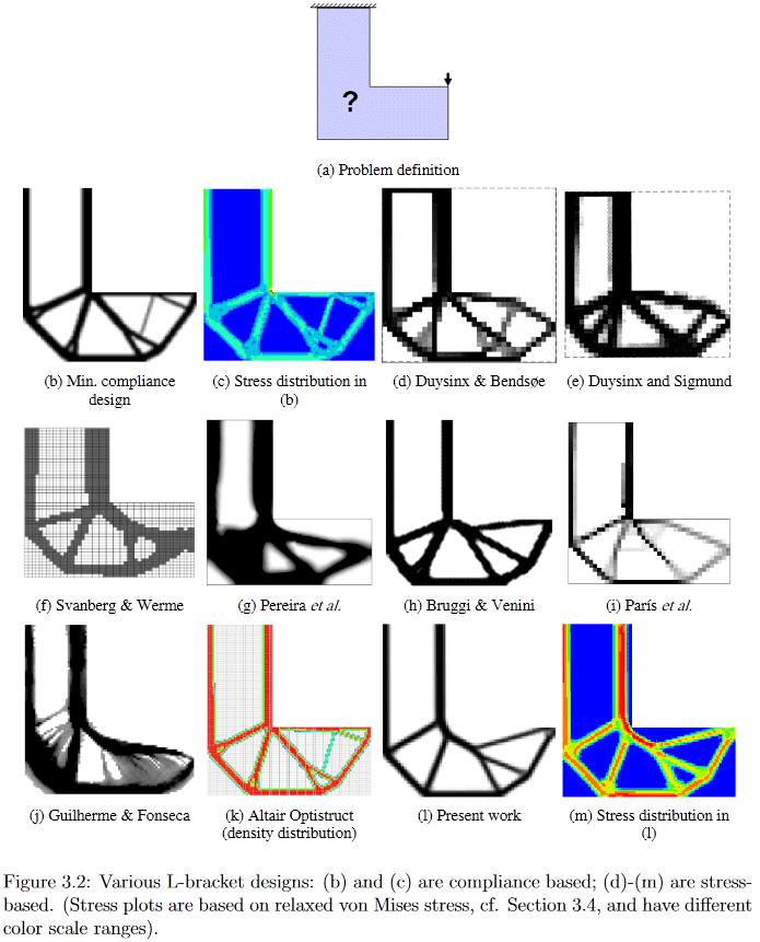
(Image from "Developments in Topology and Shape Optimization", Chau Hoai Le, 2010)
As an example, in this picture you can clearly see how very differently different algorithms generate a solution to the seemingly simple design problem of the L-shaped suspension.
So, now back to the work in question.
The authors very witty suggested solving such optimization problems by generating a candidate solution by a neural network and the subsequent evolution of the solution by gradient descent methods with respect to the objective compliance function. The compliance of the resulting structure is estimated using a differentiable physical model, which, in fact, allows the use of gradient descent. According to them (there is no code for self-checking, but I wrote to the first author of the work Stephan Hoyer and he assured that the code will be published on Github soon), this either gives the same result as the best traditional algorithms for simple tasks, or the best These algorithms, used as baselines, are complex.
Next I’ll try to describe what and how exactly the authors proposed to do, but I immediately warn that I’m not guaranteeing 100% correctness, because in addition to the extremely poor brevity of the description, I’ll also add some general “immaturity” of the article to my somewhat rusty erudition which, judging by the presence of two editions in 4 days, is being finalized ( added: at the moment, I believe that, at least, basically, everything is described correctly).
The authors, in general, follow the approach to solving such optimization problems, called the “modified SIMP method”, and described in detail in [3] “Efficient topology optimization in MATLAB using 88 lines of code”. The preprint of this work and the code associated with it can be found at http://www.topopt.mek.dtu.dk/Apps-and-software/Efficient-topology-optimization-in-MATLAB . This work is often used to start teaching students about topological optimization issues, therefore, in order to further understand it, it is recommended to be familiar with it.
In “modified SIMP”, the solution is optimized directly by modifying the pixels of the picture of physical densities. The authors of the work did not propose to modify the picture directly (although such an algorithm, with other things being equal, was a control one), but to change the parameters and input of the convolutional neural network that generates a picture of physical densities. This is how the whole method looks globally:

(Image from the publication in question)
A neural network (hereinafter referred to as NS) using the random primary input vector _beta (it, like the network weight, is a trained parameter), generates (some) picture of the solution (it works with 2D, but in 3D, I think, it can also be distributed ) The upsampling part of the well-known U-Net architecture is used as an NS generator.
Pixel values are converted to physical densities in two steps:
In short, the essence of the whole step 2 is that the unnormalized output of a completely ordinary NS turns into a properly normalized, slightly smoothed frame of the physical model (a set of physical densities of elements), to which the necessary a priori restrictions have already been applied (this is the amount of material used).
The resulting skeleton is run through a differentiable physical engine to obtain the shear vector (/ tensor?) Of the structure under load (including gravity) U. The key here is the differentiability of the engine, which allows us to obtain gradients (recall that the gradient of the function is generally tensor made up of partial derivatives of a function with respect to all its arguments.The gradient shows the direction and rate of change of the function at the current point, therefore, knowing it, you can “twist” the arguments so that the desired change occurs with the function - it decreased or increased). Such a differentiable physical engine does not need to be written from scratch - they have long existed and are well known. The authors only needed to do their pairing with neural network calculation packages, such as TensorFlow / PyTorch.
The scalar objective function c (x) to be minimized is calculated, which describes the compliance (it is the inverse of rigidity) of the resulting framework. The compliance function depends on the shift vector U obtained at the last step and the rigidity matrix of the structure K (I do not have enough knowledge of topology optimization to understand where K comes from - I assume that it seems to be directly calculated from the framework).
/ *
see also comments (1) from kxx and (2) from 350Stealth , although basic enlightenment is worth going to work [3].
* /
And then it's done. Since everything is created in an environment with automatic differentiation, at this stage we automatically get all the gradients of the objective function, which are pushed due to the differentiability of all transformations at each step back to the weights and the input vector of the generating neural network. The weights and the input vector, respectively, with their partial derivatives change, causing the necessary change - minimizing the objective function. Next, a new cycle of direct passage through the NS occurs -> application of restrictions -> miscalculation of the physical model -> calculation of the objective function -> new gradients and updating the weights. And so until the convergence of Algo.
An important point, the descriptions of which I did not find in the work, is how the total volume of the construction V0 is selected, with the help of which the candidate solution is converted to the framework in step 2. Obviously, the properties of the resulting solution extremely depend on its choice. By indirect indications (all the examples of the obtained solutions [4] have several instances differing precisely in the volume limit), I assume that they simply fix V0 on a certain grid from the range [0.05, 0.5] and then they look with their eyes at the obtained solutions with different V0. Well, for a conceptual work, this, in general, is enough, although, of course, it would be terribly interesting to see an option with the selection of this V0 as well, but, it will probably go to the next stage of development of the work.
The second important point, which I did not understand, is how they impose restrictions / requirements on the specific type of solution. Those. if you can still separate the bridge from the building thanks to the physical model (the building has full support, and the bridge is only at the boundary ends), then how to separate, say, a building of 3 floors from a building of 4 floors?
It turned out that for small (in terms of the size of the solution space = number of pixels) problems, the method gives ± the same quality of results as the best traditional methods of topological optimization, but on large ones (grid size from 2 ^ 15 or more pixels, i.e. , for example, from 128 * 256 or more) obtaining high-quality solutions by the method is more likely than the best traditional one (out of 116 tested problems, the method gave a preferred solution in 99 problems, against 66 preferred ones in the best traditional one).
Moreover, here something especially interesting begins. Traditional methods of topological optimization in large tasks suffer from the fact that in the early stages of work they quickly form a small-scale web, which then interferes with the development of large-scale structures. This leads to the fact that the result obtained is difficult / impossible to translate physically into life. Therefore, forcibly there is a whole direction in topology optimization problems that studies / comes up with methods of how to make the resulting solutions more technologically convenient.
Here, apparently, thanks to the convolution network, optimization occurs simultaneously on several spatial scales at the same time, which allows to avoid / greatly reduce the "web" and get simpler, but high-quality and technologically-friendly solutions!
In addition, again thanks to the convolution of the network, fundamentally different solutions are obtained than in standard-traditional methods.
For example, in designs:
(Image from the publication in question)
I have never seen such a use of a neural network. Typically, neural networks are used to get some very tricky and complex function y = F (x, theta) (where x is the argument, and theta are the tunable parameters), which can do something useful. For example, if x is a picture from a car’s camera, then the y value of the function can be, for example, a sign of whether there is a pedestrian in dangerously close to the car. Those. here it is important that the particular form of the function itself, which is repeatedly used to solve a problem, is valuable.
Here, the neural network is used as a cunning repository-modifier-adjuster of parameters of some physical model, which, due to its very architecture, imposes certain restrictions on the values and variations of changes in these parameters (in fact, the examples under the heading Pixel-LBFGS are an attempt to optimize pixels directly, not using a neural network to generate them, the results are visible, the NS is important). This is where the convolution of the used neural network becomes critically important, because it is its architecture that allows you to “catch” the concept of transfer invariance and a bit of rotation (imagine that you recognize text from a picture - it’s important for you to extract the text and it doesn’t matter which parts of the picture, it is located and how it is rotated - that is, you need the invariance of the transfer and rotation). In this problem, some kind of physical stick, which is a unit of structure and many of which we optimize, still remains it regardless of its position and orientation in space.
A classic fully-connected network, for example, would probably not work here (just as good), because its architecture allows too much / small (well, yes, such dualism, how to look). At the same time, despite the fact that the NS remains here the very very tricky and complex function y = F (x, theta), in this task we ultimately do not give a damn about its argument x or its parameters theta , and how the function will be used. We are only concerned about its single value y, which is obtained in the process of optimizing one specific objective function for one specific physical model, in which {x, theta} are just configurable parameters!
This, in my opinion, is awesomely cool and new idea! (although, of course, then, as always, it may turn out that Schmidhuber described it back in the early 90s, but we will wait and see)
In general, the meaning of the method is somewhat reminiscent of reinforced learning - there the NS is used, roughly speaking, as a “repository of experience” of an agent acting in a certain environment, which is updated as the environment receives feedback on the agent’s actions. Only there, this very “repository of experience" is constantly used for making new decisions by the agent, and here it is just a repository of parameters of the physical model, from which we are only interested in the only one final result of optimization.
Well, the last. An interesting moment caught my eye.
This is how optimal solutions for the task of a multi-story building look like:
(Image from the publication in question)
And like this:

arranged inside the fantastic Sagrada Familia, the Temple of the Sagrada Familia, located in Barcelona, Spain, which was “designed” by the brilliant Antonio Gaudi.
I thank the first author of the article, Stephan Hoyer, for prompt assistance in explaining some obscure details of the work, as well as for the Habr participants who made their additions and / or useful provocative ideas.
[1] option for determining the structural / topological optimization problem
[2] "Developments in Topology and Shape Optimization"
[3] Andreassen, E., Clausen, A., Schevenels, M., Lazarov, BS, and Sigmund, O. Efficient topology optimization in MATLAB using 88 lines of code. Structural and Multidisciplinary Optimization, 43 (1): 1–16, 2011. A preprint of this work and code are available at http://www.topopt.mek.dtu.dk/Apps-and-software/Efficient-topology-optimization-in -MATLAB
[4] examples of solutions
Last update of the article 2019.10.05 12:50
What are you talking about? What is the task of topological optimization?
Just imagine what you need, for example, to design a thread of a bridge, a multi-story building, an airplane wing, a turbine blade, or whatever. Usually, this is solved by finding a specialist, for example, an architect, who would use his knowledge of matan, sopromat, target area, as well as his experience, intuition, test layouts, etc. etc. would create the desired project. It is important here that this received project would be good only to the best of this specialist. And this, obviously, is not always enough. Therefore, when computers became powerful enough, we began to try to shift such tasks to them. For
Such tasks are called "structural optimization problems", i.e. generating an optimal design of load-bearing mechanical structures [1]. A subsection of structural optimization problems are topological optimization problems (in fact, the work in question is specifically focused on them, but this is absolutely not the point, and more on that later). A typical topological optimization problem looks something like this: for a given concept (bridge, house, etc.) in space in two or three dimensions, having specific limitations in the form of materials, technologies and other requirements, having some external loads, you need to design an optimal structure that will hold loads and satisfy constraints.
- "Designing" essentially means finding / describing a subspace of the source space that needs to be filled with building material.
- Optimality can be expressed, for example, in the form of a requirement to minimize the total weight of the structure under restrictions in the form of the maximum allowable stresses in the material and possible displacements at given loads.
To solve this problem on a computer, the target solution space is sampled into a set of finite elements (pixels for 2D and voxels for 3D) and then, using some algorithm, the computer decides whether to fill this individual element with material or leave it empty?
(Image from "Developments in Topology and Shape Optimization", Chau Hoai Le, 2010)
So, already from the statement of the problem it is clear that its solution is quite a big splinter for scientists. I can offer those who wish some details, for example, look at a very old one (2010, which is still a lot for an actively developing field), but a rather detailed and easy-to-google Chau Hoai Le dissertation entitled "Developments in Topology and Shape Optimization" [2], where I stole the top and bottom pictures.
(Image from "Developments in Topology and Shape Optimization", Chau Hoai Le, 2010)
As an example, in this picture you can clearly see how very differently different algorithms generate a solution to the seemingly simple design problem of the L-shaped suspension.
So, now back to the work in question.
The authors very witty suggested solving such optimization problems by generating a candidate solution by a neural network and the subsequent evolution of the solution by gradient descent methods with respect to the objective compliance function. The compliance of the resulting structure is estimated using a differentiable physical model, which, in fact, allows the use of gradient descent. According to them (there is no code for self-checking, but I wrote to the first author of the work Stephan Hoyer and he assured that the code will be published on Github soon), this either gives the same result as the best traditional algorithms for simple tasks, or the best These algorithms, used as baselines, are complex.
Method
Next I’ll try to describe what and how exactly the authors proposed to do, but I immediately warn that I’m not guaranteeing 100% correctness, because in addition to the extremely poor brevity of the description, I’ll also add some general “immaturity” of the article to my somewhat rusty erudition which, judging by the presence of two editions in 4 days, is being finalized ( added: at the moment, I believe that, at least, basically, everything is described correctly).
The authors, in general, follow the approach to solving such optimization problems, called the “modified SIMP method”, and described in detail in [3] “Efficient topology optimization in MATLAB using 88 lines of code”. The preprint of this work and the code associated with it can be found at http://www.topopt.mek.dtu.dk/Apps-and-software/Efficient-topology-optimization-in-MATLAB . This work is often used to start teaching students about topological optimization issues, therefore, in order to further understand it, it is recommended to be familiar with it.
In “modified SIMP”, the solution is optimized directly by modifying the pixels of the picture of physical densities. The authors of the work did not propose to modify the picture directly (although such an algorithm, with other things being equal, was a control one), but to change the parameters and input of the convolutional neural network that generates a picture of physical densities. This is how the whole method looks globally:
(Image from the publication in question)
Step 1, candidate generation
A neural network (hereinafter referred to as NS) using the random primary input vector _beta (it, like the network weight, is a trained parameter), generates (some) picture of the solution (it works with 2D, but in 3D, I think, it can also be distributed ) The upsampling part of the well-known U-Net architecture is used as an NS generator.
Step 2, applying restrictions and converting a candidate to a physical model framework
Pixel values are converted to physical densities in two steps:
- First, in one step, the issue of normalizing the non-normalized values of the generated pixels is solved (the NS is designed so that it outputs the so-called logits - values in the range (-inf, + inf)) and applying restrictions on the total amount of the resulting solution. For this, a sigmoid is applied element-wise to the picture, the argument of which is shifted by a constant depending on the image being transformed and the volume of the desired solution (the value of this bias constant is selected by binary search so that the total volume of the densities obtained in this way is equal to a certain predetermined volume V0). A detailed analysis of this stage, see the comment );
- Next, the resulting normalized picture of the densities of the structure is processed by the so-called a density filter with a radius of 2. In more well-known terms, this filter is nothing more than a normal weighted average of neighboring points in the picture. The weights in this filter (filter core) can be represented as the values of the height of points located on the surface of a regular cone, which lies with its base on the plane so that its vertex is at the current point, so the authors call it cone-filter (in more detail on this topic see the description of density filter in chapter 2.3 Filtering of [3]).
In short, the essence of the whole step 2 is that the unnormalized output of a completely ordinary NS turns into a properly normalized, slightly smoothed frame of the physical model (a set of physical densities of elements), to which the necessary a priori restrictions have already been applied (this is the amount of material used).
Step 3, evaluation of the resulting frame physical model
The resulting skeleton is run through a differentiable physical engine to obtain the shear vector (/ tensor?) Of the structure under load (including gravity) U. The key here is the differentiability of the engine, which allows us to obtain gradients (recall that the gradient of the function is generally tensor made up of partial derivatives of a function with respect to all its arguments.The gradient shows the direction and rate of change of the function at the current point, therefore, knowing it, you can “twist” the arguments so that the desired change occurs with the function - it decreased or increased). Such a differentiable physical engine does not need to be written from scratch - they have long existed and are well known. The authors only needed to do their pairing with neural network calculation packages, such as TensorFlow / PyTorch.
Step 4, calculating the value of the objective function for the wireframe / candidate
The scalar objective function c (x) to be minimized is calculated, which describes the compliance (it is the inverse of rigidity) of the resulting framework. The compliance function depends on the shift vector U obtained at the last step and the rigidity matrix of the structure K (I do not have enough knowledge of topology optimization to understand where K comes from - I assume that it seems to be directly calculated from the framework).
/ *
see also comments (1) from kxx and (2) from 350Stealth , although basic enlightenment is worth going to work [3].
* /
And then it's done. Since everything is created in an environment with automatic differentiation, at this stage we automatically get all the gradients of the objective function, which are pushed due to the differentiability of all transformations at each step back to the weights and the input vector of the generating neural network. The weights and the input vector, respectively, with their partial derivatives change, causing the necessary change - minimizing the objective function. Next, a new cycle of direct passage through the NS occurs -> application of restrictions -> miscalculation of the physical model -> calculation of the objective function -> new gradients and updating the weights. And so until the convergence of Algo.
An important point, the descriptions of which I did not find in the work, is how the total volume of the construction V0 is selected, with the help of which the candidate solution is converted to the framework in step 2. Obviously, the properties of the resulting solution extremely depend on its choice. By indirect indications (all the examples of the obtained solutions [4] have several instances differing precisely in the volume limit), I assume that they simply fix V0 on a certain grid from the range [0.05, 0.5] and then they look with their eyes at the obtained solutions with different V0. Well, for a conceptual work, this, in general, is enough, although, of course, it would be terribly interesting to see an option with the selection of this V0 as well, but, it will probably go to the next stage of development of the work.
The second important point, which I did not understand, is how they impose restrictions / requirements on the specific type of solution. Those. if you can still separate the bridge from the building thanks to the physical model (the building has full support, and the bridge is only at the boundary ends), then how to separate, say, a building of 3 floors from a building of 4 floors?
How it works?
It turned out that for small (in terms of the size of the solution space = number of pixels) problems, the method gives ± the same quality of results as the best traditional methods of topological optimization, but on large ones (grid size from 2 ^ 15 or more pixels, i.e. , for example, from 128 * 256 or more) obtaining high-quality solutions by the method is more likely than the best traditional one (out of 116 tested problems, the method gave a preferred solution in 99 problems, against 66 preferred ones in the best traditional one).
Moreover, here something especially interesting begins. Traditional methods of topological optimization in large tasks suffer from the fact that in the early stages of work they quickly form a small-scale web, which then interferes with the development of large-scale structures. This leads to the fact that the result obtained is difficult / impossible to translate physically into life. Therefore, forcibly there is a whole direction in topology optimization problems that studies / comes up with methods of how to make the resulting solutions more technologically convenient.
Here, apparently, thanks to the convolution network, optimization occurs simultaneously on several spatial scales at the same time, which allows to avoid / greatly reduce the "web" and get simpler, but high-quality and technologically-friendly solutions!
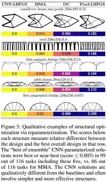
In addition, again thanks to the convolution of the network, fundamentally different solutions are obtained than in standard-traditional methods.
For example, in designs:
- cantilever beam method found a solution of only 8 components, while the best traditional - 18.
- thin support bridge method selected one support with a tree-like branching pattern, while the traditional one - two supports
- The roof method uses columns, while the traditional method uses a branching pattern. Etc.
(Image from the publication in question)
What is so special about this work?
I have never seen such a use of a neural network. Typically, neural networks are used to get some very tricky and complex function y = F (x, theta) (where x is the argument, and theta are the tunable parameters), which can do something useful. For example, if x is a picture from a car’s camera, then the y value of the function can be, for example, a sign of whether there is a pedestrian in dangerously close to the car. Those. here it is important that the particular form of the function itself, which is repeatedly used to solve a problem, is valuable.
Here, the neural network is used as a cunning repository-modifier-adjuster of parameters of some physical model, which, due to its very architecture, imposes certain restrictions on the values and variations of changes in these parameters (in fact, the examples under the heading Pixel-LBFGS are an attempt to optimize pixels directly, not using a neural network to generate them, the results are visible, the NS is important). This is where the convolution of the used neural network becomes critically important, because it is its architecture that allows you to “catch” the concept of transfer invariance and a bit of rotation (imagine that you recognize text from a picture - it’s important for you to extract the text and it doesn’t matter which parts of the picture, it is located and how it is rotated - that is, you need the invariance of the transfer and rotation). In this problem, some kind of physical stick, which is a unit of structure and many of which we optimize, still remains it regardless of its position and orientation in space.
A classic fully-connected network, for example, would probably not work here (just as good), because its architecture allows too much / small (well, yes, such dualism, how to look). At the same time, despite the fact that the NS remains here the very very tricky and complex function y = F (x, theta), in this task we ultimately do not give a damn about its argument x or its parameters theta , and how the function will be used. We are only concerned about its single value y, which is obtained in the process of optimizing one specific objective function for one specific physical model, in which {x, theta} are just configurable parameters!
This, in my opinion, is awesomely cool and new idea! (although, of course, then, as always, it may turn out that Schmidhuber described it back in the early 90s, but we will wait and see)
In general, the meaning of the method is somewhat reminiscent of reinforced learning - there the NS is used, roughly speaking, as a “repository of experience” of an agent acting in a certain environment, which is updated as the environment receives feedback on the agent’s actions. Only there, this very “repository of experience" is constantly used for making new decisions by the agent, and here it is just a repository of parameters of the physical model, from which we are only interested in the only one final result of optimization.
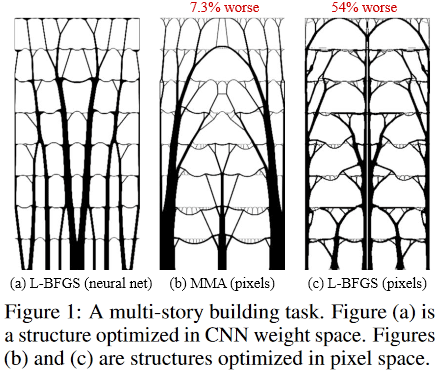
Well, the last. An interesting moment caught my eye.
This is how optimal solutions for the task of a multi-story building look like:
(Image from the publication in question)
And like this:
arranged inside the fantastic Sagrada Familia, the Temple of the Sagrada Familia, located in Barcelona, Spain, which was “designed” by the brilliant Antonio Gaudi.
Acknowledgments
I thank the first author of the article, Stephan Hoyer, for prompt assistance in explaining some obscure details of the work, as well as for the Habr participants who made their additions and / or useful provocative ideas.
[1] option for determining the structural / topological optimization problem
[2] "Developments in Topology and Shape Optimization"
[3] Andreassen, E., Clausen, A., Schevenels, M., Lazarov, BS, and Sigmund, O. Efficient topology optimization in MATLAB using 88 lines of code. Structural and Multidisciplinary Optimization, 43 (1): 1–16, 2011. A preprint of this work and code are available at http://www.topopt.mek.dtu.dk/Apps-and-software/Efficient-topology-optimization-in -MATLAB
[4] examples of solutions
Last update of the article 2019.10.05 12:50
All Articles