Synthesis of a controller by the inverse dynamics problem method
In control problems, there are cases when the law of motion of a controlled object is known and it is necessary to develop a regulator with certain characteristics. Sometimes the task is complicated by the fact that the equations describing the controlled object turn out to be nonlinear, which complicates the construction of the controller. In this regard, several methods have been developed to take into account nonlinear structural features of the control object, one of which is the inverse dynamics problem method.
The method of the inverse problem of dynamics naturally arises when you try to "convert" one dynamic system to another, when the developer has two equations, one of which describes an existing controlled system, and the other expresses the law of motion of that very controlled system, turning it into something useful. The law may look different, but the main thing is that it be physically feasible. This may be the law of the sinusoidal voltage change at the output of the generator or the automatic frequency control system, the law of the speed of rotation of the turbine or the movement of the printer’s cradle, or even it can be the X, Y coordinates of the pencil lead used by the manipulator to sign the postcards.
However, it is possible to “impose” your control law that fits into the framework of physical realizability and controllability of an object and this is often not the most difficult part of development. But the fact that the method under consideration makes it quite easy to take into account the nonlinearity and multidimensionality of the object in my opinion increases its attractiveness. By the way, here you can notice the connection with the feedback non-linearity compensation method [1].
It is known that in some cases correctly formed nonlinear controllers even when controlling a linear system give better control characteristics in comparison with linear controllers [2]. An example is a regulator that reduces the damping coefficient of a system with an increase in the error of working out a command and increases it as the error decreases, which leads to an improvement in the quality of the transient process.
Generally speaking, the topic of control associated with the need to take into account nonlinearities has long attracted the attention of scientists and engineers, since most real objects are nevertheless described by nonlinear equations. Here are some examples of non-linearities commonly found in technology:
The general statement of the problem is as follows. Let there be a control object that can be described as an nth-order differential equation
in which there is a disturbance (this may be the noise of the measuring device, external random influence, vibration, etc.) and the control signal (in technology, control is most often carried out using voltage). In this case, for simplicity of perception, we consider a one-dimensional control object, which includes one perturbation. In the general case, these quantities are vectorial. It is understood that phase variables that describe the state of the control object, disturbances and management depend on time, but this fact is not displayed for simplicity of perception. Expression (1) may contain non-linearities, as well as be non-stationary, i.e. whose parameters clearly change over time. An example of an unsteady equation can be the number of uranium nuclei in a reactor, which is constantly decreasing as a result of the decay reaction, which leads to a continuous change in the optimal control law of moderator rods.
The controller is constructed in such a way as to work out a previously known control law, which can be described by a differential order equation, not lower than the order of equation (1), which describes the control object:
Where - the control signal and its derivatives in an amount that allows you to fully describe the required control law. So, for the stabilization system, it is not necessary to measure the derivatives of control. For a tracking system for a ramp input signal, it is sufficient to measure the first derivative. To track the quadratically varying signal, you have to add a second derivative, and so on. It should be noted that this signal is fed to the input of the regulator, in contrast to the signal entering the control object from the regulator. This equation can also be non-linear as well as non-stationary.
To determine the desired control signal we express from (2) the highest derivative
and substitute the resulting expression instead in equation (1), while expressing the control:
From expression (3), it becomes clear that in order to create the required control signal, it is necessary to measure, in addition to external disturbances (if their influence is significant), as the controlled quantity itself , and all its derivatives up to order inclusive, which may cause some difficulties. Firstly, the higher derivatives may not be available for measurement directly, as we say the derivative of acceleration, as a result of which it is necessary to resort to the operation of differentiation, programmatically or circuitry. And, as you know, they try to avoid this because of the increase in noise. Secondly, measurements inevitably contain noise, and this forces one to resort to filtering. Any filter is a dynamic or, in other words, an inertial element, which means the presence of a derivative with the equation. Consequently, the order of the entire control system in the general case will increase by a number equal to the sum of the orders of equations describing all filter meters. That is, if we control a second-order object and use second-order filters in each measurement channel (that is, only two second-order filters) for measuring the output quantity and its derivative, then the order of the control system will increase by four. Of course, if the filter time constants are sufficiently small, then the influence of smoothing elements can be neglected. But in any case, they will bring the so-called small dynamic parameters into the system and their combined contribution can affect the stability of the control system as a whole [2]. It should also be understood that this method allows you to specify control only in the transition process and is not associated with optimization by any criterion of control quality.
The relationship of the controller and the control object can be described by the following scheme:

Consider an example of a controller synthesis for controlling a self-oscillating system. This is a fictitious example that explains the essence of the method well. Suppose you want to control a system whose equation is as follows:
The law of management should be as follows:
Where - our driving control signal (setpoint). That is, in fact, we want to "turn" our generator with non-linearity into a linear oscillatory link. It should be noted that in the same [2] this system is a stabilization system, since the output seeks to repeat the input signal , that is, stabilizes the system output at a given constant level that can be displayed as
It is important that the input signal was constant or slowly changing (so slowly that the lag error from fit into our requirements for accuracy) with a value or piecewise constant function, since the whole system has astatism of the 0th order (that is, is static) and for any constantly changing setting signal a dynamic error will certainly appear at the system output, which will look like adding a certain constant value to the output value that monotonically depends on the rate of change of the control action. This feature will be eliminated in the future.
So, we express the highest derivative from equation (5):
and substitute it in (4), expressing :
This is the control signal, which will be formed by the regulator from the desired control signal . From (6) also follows the need to measure the output quantity and its first derivative.
Van der Pol oscillator self-oscillations with parameters look like this:

Let us have a “step” type signal:

and we want the system to repeat it.
We feed it to the input of the oscillator and see the response:

Under the action of the input single signal, only a small constant bias was added to the oscillations of the oscillator.
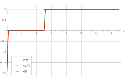
Suppose now that we need to obtain such an oscillator response to a master signal that would correspond to the reaction of the vibrational link (5) with a time constant and damping factor . Response of such an oscillatory link per unit step is presented below:

Now let’s give the control signal to the oscillator described by expression (6):
It can be seen that the oscillator behaves in accordance with the required law. Let's look at the control signal :

The figure shows a significant surge at the time of the transition process. In a real system, most likely, either the system will enter saturation (destruction), or in order to prevent this, we will have to limit the input signal. We take this into account by limiting the amplitude of the control action at the level 15. The control signal now looks like this:

and the oscillator output is like this:
The consequence of the signal limitation is a large transient error, which, depending on the desired properties of the system, can be quite significant. With an increase in the required time constant, transient emissions decrease. You need to be careful that the maximum control signal in the steady state (which on this graph starts from about the sixth second) is not limited, otherwise there will be an endless transient and the system will not work out the task. Regulator gain, i.e. control signal ratio at the regulator output determined by the parameters of the controlled system, namely the factor .
Now let’s feed the oscillator with such a linearly changing signal:

The reaction of the vibrational link:
and oscillator:
It is seen that a constant lag has appeared - a dynamic error, because the system is designed to track only a constant setting signal . In order to be able to track a linearly varying signal, it is necessary to evaluate the rate of its change and take it into account in the controller. To do this, we compose the required control law as follows:
Where - error tracking the master signal by the oscillator.
We also express the highest derivative from (7), substitute it into the equation of the control object (4) and get the control signal:
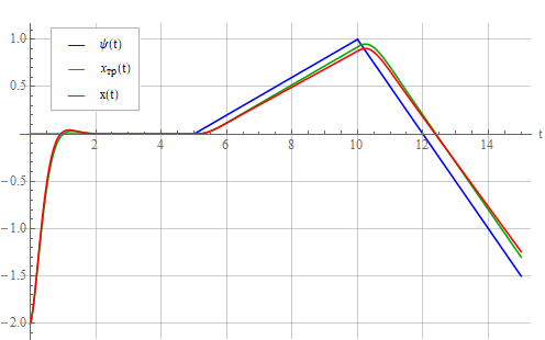
In the new structure of the regulator corresponding to expression (8), the rate of change of the set action . We look at the output of the system when a linearly varying setpoint is applied to the input:

Oscillator tracks the set signal .
But this is a completely synthetic example. In reality, there will be a system whose structure is probably not identified accurately enough - this time. We will also determine the system parameters with a certain error - these are two. Control includes phase variables that will have to be measured with some kind of noise are three. And the parameters of the system can float away over time, that is, a stationary system over a sufficiently long period of time can show non-stationarity. Although it’s more correct to say so - on a fairly short time interval, a non-stationary system may seem stationary. In this example, we assume that the system is identified with sufficient accuracy and its change in time is very insignificant. Then, for clarity, we rewrite the expression for controller (6) as follows:
Where - measured controlled value and its derivative; - identified natural frequency and non-linear attenuation coefficient, respectively.
Add a 10% error in the identification of the oscillator parameters by setting . Let's look at the result:

It can be seen from the figure that a static error appeared, which grows with an increase in the identification error and in steady state is independent of error . But the latter affects the deviation of the oscillator transient from that for the ideal oscillatory link. You can try to do the same as in the design of PID controllers ( Habr and not Habr ) - add the integral of the error to the control signal (without forgetting about the integral saturation once or twice ). But for now, we omit this question and consider expression (9), where it can be seen that the lower the natural frequency compared to the required time constant , the smaller the influence of the identification error of the same . Reduce from 0.125 to 0.05. Static error also decreased:
Now let’s try to compensate for the static error by adding the integral of the error to the controller (as in the PI controller). Expression (9) will turn into
Where - coefficient of the integral component; - current time.
The integral here is formally written as explaining the general idea, rather than the mathematical description of a specific algorithm, since in a real controller it is necessary to take measures to limit the accumulated error, otherwise problems with the transient can occur. Let us take a look at the reaction of the system under the action of the resulting regulator corresponding to expression (10):
It can be seen from the figure that the static error decreases over time, but the transient process is delayed. By analogy with the PID controller, you can try to add proportional and differentiating components. The result was as follows (the coefficients were not carefully chosen):
Naturally, the addition of the integral and differential components is no longer part of the inverse dynamics problem method, but implements a certain method for optimizing the transient process.
Let us analyze the effect of noise measurements of variables . Again, we feed a step to the system input and look at the output in the absence of any noise (there is still the same 10% identification error):
Now add to the measurements white Gaussian noises with zero expectation and equal variances passed through aperiodic links with time constants that simulate a measuring sensor + low-pass filter . One of the resulting noise implementations:
Now the system output also began to make noise:
as a result of a noisy control signal:
Take a look at the error working out the task:
Let's try to increase the time constants of the sensors and look at the system output again:
Significant fluctuations appeared - the result of the very unaccounted for small dynamic parameters [2] describing the sensors (their inertia). These dynamic parameters make noise filtering difficult, forcing to describe sensors with “large” time constants, which, generally speaking, cannot always give a positive result.
This is a more real case of applying the inverse dynamics problem method. Consider the organization of control of a DC collector motor with excitation from permanent magnets (ala Chinese motors from toys). In principle, the topic of controlling such engines is well covered and does not cause any particular difficulties. The inverse dynamics problem method will be used by and large to compensate for non-linearity in the engine dynamics equation. We assume that the engine itself could be described by linear differential equations, but there is a significant influence of the nonlinear viscous friction of the shaft, proportional to the square of its rotation speed. The equation of the electromechanical system is as follows:
Where - angular velocity of rotation of the shaft; - moment of inertia of the entire rotating system (anchors with attached load); - a machine constant, defined for a specific engine design, relating magnetic flux and shaft rotation speed; - magnetic flux, which can roughly be considered constant for a particular motor design in the range of operating currents (but in the case of high currents non-linearly dependent on the winding current); - current through the armature winding; - coefficient of linear viscous friction; - coefficient of nonlinear viscous friction; - load moment; - inductance of the armature winding; - voltage applied to the winding; - coefficient of counter-EMF, constant for a specific engine design; - resistance of the armature winding.In principle, it would be sufficient to get along with only non-linear viscous friction, but it was decided to present the non-linear dependence of friction on the shaft rotation speed as a binomial for more generality.
We will try to make such a regulator by the method of the inverse problem of dynamics, so that the dynamics of the error in fulfilling the task in terms of speed by the engine corresponds to that for the vibrational link described by the expression
Where is the angular velocity of rotation of the motor shaft; - speed setting.
Equation (12) could be compiled using the error of working out the command as a dynamic variable :
but then the terms with derivatives of the setpoint would appear in the equation, as can be seen from the expression
This, in turn, would increase the fluctuation component of the error. And since we want the system to work out only a constant, abruptly changing set point (that is, considering its speed, acceleration and all subsequent derivatives to be zero), then we need to track the maximum error in position, not taking into account its derivatives, or, if it is easier to understand , with zero derivatives of the error, which would lead to expression (12).
To obtain an expression that finally describes the regulator, it is necessary to reduce the system of two first-order equations (11) to one second-order equation. To do this, we differentiate the first equation (11) in time (assuming that the load moment is unchanged):
and substitute into it the expression from the second equation of system (11) , which gives a second-order equation
Substituting into expression (13) obtained from (12) we can find the required control to implement the desired law of motion (12):
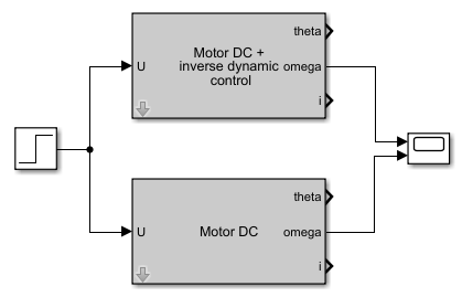
We apply to the inputs of two engines, one of which is supplemented by a regulator implemented according to the principle of the inverse dynamic problem, a step with a unit amplitude in accordance with the following scheme:
and see the dependence of the rotational speed of the motor shafts on time:
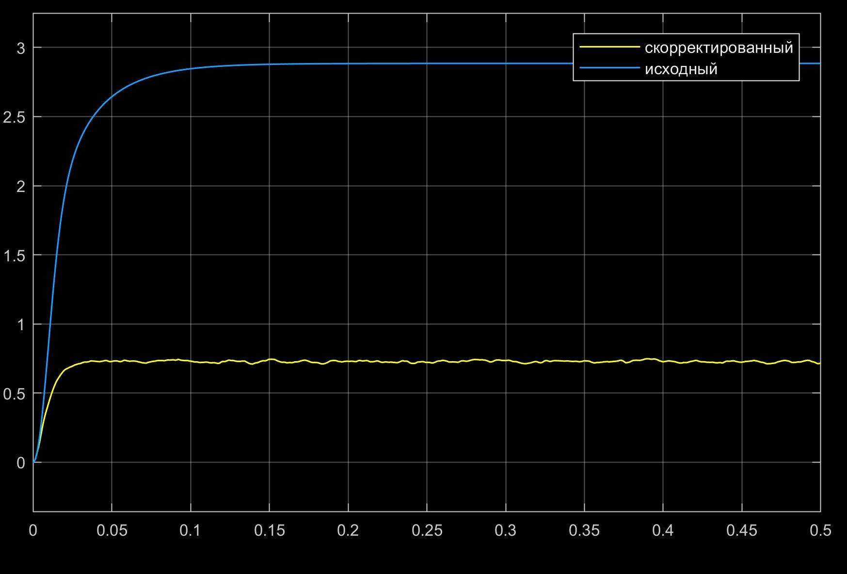
Reaction to a step with an amplitude of 10 volts:
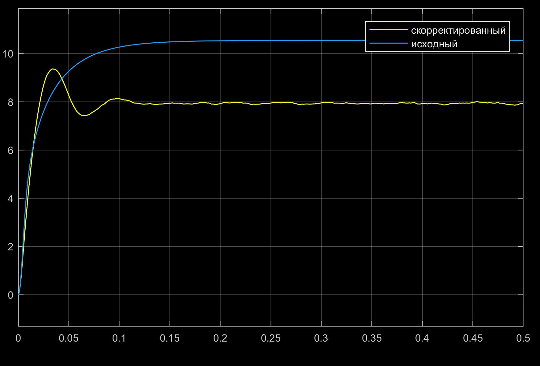
From the figures, a nonlinear dependence of the oscillation index of the initial system on the amplitude of the input signal is visible.
Now compare two engines with PID controllers, the structural diagram of which is shown in the following figure:

Frequencies of rotation of shaft of engines:

and larger:
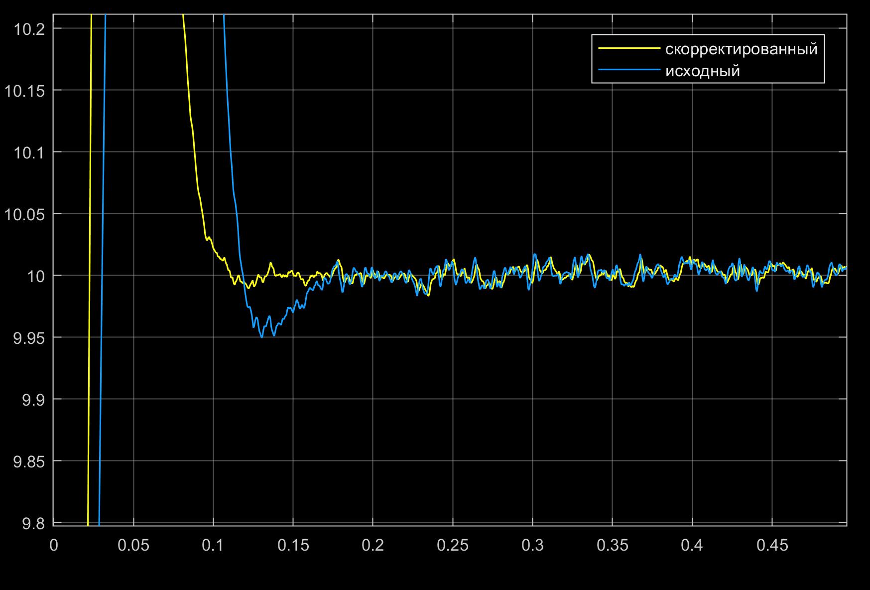
It can be seen from the figures that, thanks to the PID controller constructed using the inverse dynamic problem method, the system response to the step-by-step control signal was accelerated, which could not be achieved using the conventional PID controller due to the non-linearity in the control object. However, the use of variable coefficients of the PID controller would probably solve this problem better and make the system more robust. But this is a completely different story.
The article considered a method that allows you to build a controller for controlling non-linear systems, which was shown by examples of controls of the Van der Pol oscillator and a DC motor.
The main advantages of this method include:
However, this method also has a number of significant disadvantages :
In general, this is a rather interesting method, but by comparing its implementation for controlling a DC motor (using a PID controller) with a motor controlled only by a PID controller, it became clear that significant buns could not be obtained from it. But the structure of the control device is much more complicated, forcing, among other things, to struggle with differentiation noises on the one hand, and preventing the stability boundary from reaching the other hand. Perhaps it is with this that a small number of works on this topic are connected. One of the possible applications of the method of the inverse problem of dynamics can be the construction of reference (ideal) trajectories of systems for comparison with trajectories corresponding to various controllers, for example, linear or linearized.
1. Kim D.P. Theory of automatic control. T.2. Multidimensional, nonlinear, optimal and adaptive systems: Textbook. allowance.- M .: FIZMATLIT, 2004 .-- 464 p.
2. Boychuk L.M. The method of structural synthesis of nonlinear automatic control systems. M., "Energy", 1971.
3. Non-stationary automatic control systems: analysis, synthesis and optimization / Ed. K.A. Pupkova and N.D. Egupova. - M .: Publishing house of MGTU im. N.E. Bauman, 2007 .-- 632 p.
Introduction
The method of the inverse problem of dynamics naturally arises when you try to "convert" one dynamic system to another, when the developer has two equations, one of which describes an existing controlled system, and the other expresses the law of motion of that very controlled system, turning it into something useful. The law may look different, but the main thing is that it be physically feasible. This may be the law of the sinusoidal voltage change at the output of the generator or the automatic frequency control system, the law of the speed of rotation of the turbine or the movement of the printer’s cradle, or even it can be the X, Y coordinates of the pencil lead used by the manipulator to sign the postcards.
However, it is possible to “impose” your control law that fits into the framework of physical realizability and controllability of an object and this is often not the most difficult part of development. But the fact that the method under consideration makes it quite easy to take into account the nonlinearity and multidimensionality of the object in my opinion increases its attractiveness. By the way, here you can notice the connection with the feedback non-linearity compensation method [1].
It is known that in some cases correctly formed nonlinear controllers even when controlling a linear system give better control characteristics in comparison with linear controllers [2]. An example is a regulator that reduces the damping coefficient of a system with an increase in the error of working out a command and increases it as the error decreases, which leads to an improvement in the quality of the transient process.
Generally speaking, the topic of control associated with the need to take into account nonlinearities has long attracted the attention of scientists and engineers, since most real objects are nevertheless described by nonlinear equations. Here are some examples of non-linearities commonly found in technology:
 |  |
 |  |
 |  |
 |  |
The general statement of the problem is as follows. Let there be a control object that can be described as an nth-order differential equation
in which there is a disturbance (this may be the noise of the measuring device, external random influence, vibration, etc.) and the control signal (in technology, control is most often carried out using voltage). In this case, for simplicity of perception, we consider a one-dimensional control object, which includes one perturbation. In the general case, these quantities are vectorial. It is understood that phase variables that describe the state of the control object, disturbances and management depend on time, but this fact is not displayed for simplicity of perception. Expression (1) may contain non-linearities, as well as be non-stationary, i.e. whose parameters clearly change over time. An example of an unsteady equation can be the number of uranium nuclei in a reactor, which is constantly decreasing as a result of the decay reaction, which leads to a continuous change in the optimal control law of moderator rods.
The controller is constructed in such a way as to work out a previously known control law, which can be described by a differential order equation, not lower than the order of equation (1), which describes the control object:
Where - the control signal and its derivatives in an amount that allows you to fully describe the required control law. So, for the stabilization system, it is not necessary to measure the derivatives of control. For a tracking system for a ramp input signal, it is sufficient to measure the first derivative. To track the quadratically varying signal, you have to add a second derivative, and so on. It should be noted that this signal is fed to the input of the regulator, in contrast to the signal entering the control object from the regulator. This equation can also be non-linear as well as non-stationary.
To determine the desired control signal we express from (2) the highest derivative
and substitute the resulting expression instead in equation (1), while expressing the control:
$$ display $$ \ begin {matrix} {u = F \ left ({{f}} ({{x} ^ {(n-1)}}, {{x} ^ {(n-2)}} , \ ... \, \ x, \ psi (t), \ {{\ psi} ^ {(1)}}, \ ..., {{\ psi} ^ {(k)}}, t) , \\ \ quad \ quad \ quad \ quad {{x} ^ {(n-1)}}, {{x} ^ {(n-2)}}, \ ... \, \ x, \ { {\ xi}}, t \ right).} & \ quad \ quad \ quad (3) \ end {matrix} $$ display $$
From expression (3), it becomes clear that in order to create the required control signal, it is necessary to measure, in addition to external disturbances (if their influence is significant), as the controlled quantity itself , and all its derivatives up to order inclusive, which may cause some difficulties. Firstly, the higher derivatives may not be available for measurement directly, as we say the derivative of acceleration, as a result of which it is necessary to resort to the operation of differentiation, programmatically or circuitry. And, as you know, they try to avoid this because of the increase in noise. Secondly, measurements inevitably contain noise, and this forces one to resort to filtering. Any filter is a dynamic or, in other words, an inertial element, which means the presence of a derivative with the equation. Consequently, the order of the entire control system in the general case will increase by a number equal to the sum of the orders of equations describing all filter meters. That is, if we control a second-order object and use second-order filters in each measurement channel (that is, only two second-order filters) for measuring the output quantity and its derivative, then the order of the control system will increase by four. Of course, if the filter time constants are sufficiently small, then the influence of smoothing elements can be neglected. But in any case, they will bring the so-called small dynamic parameters into the system and their combined contribution can affect the stability of the control system as a whole [2]. It should also be understood that this method allows you to specify control only in the transition process and is not associated with optimization by any criterion of control quality.
The relationship of the controller and the control object can be described by the following scheme:
Van der Pol Oscillator Control
Consider an example of a controller synthesis for controlling a self-oscillating system. This is a fictitious example that explains the essence of the method well. Suppose you want to control a system whose equation is as follows:
The law of management should be as follows:
Where - our driving control signal (setpoint). That is, in fact, we want to "turn" our generator with non-linearity into a linear oscillatory link. It should be noted that in the same [2] this system is a stabilization system, since the output seeks to repeat the input signal , that is, stabilizes the system output at a given constant level that can be displayed as
It is important that the input signal was constant or slowly changing (so slowly that the lag error from fit into our requirements for accuracy) with a value or piecewise constant function, since the whole system has astatism of the 0th order (that is, is static) and for any constantly changing setting signal a dynamic error will certainly appear at the system output, which will look like adding a certain constant value to the output value that monotonically depends on the rate of change of the control action. This feature will be eliminated in the future.
So, we express the highest derivative from equation (5):
and substitute it in (4), expressing :
This is the control signal, which will be formed by the regulator from the desired control signal . From (6) also follows the need to measure the output quantity and its first derivative.
Van der Pol oscillator self-oscillations with parameters look like this:
Let us have a “step” type signal:
and we want the system to repeat it.
We feed it to the input of the oscillator and see the response:
Under the action of the input single signal, only a small constant bias was added to the oscillations of the oscillator.
Suppose now that we need to obtain such an oscillator response to a master signal that would correspond to the reaction of the vibrational link (5) with a time constant and damping factor . Response of such an oscillatory link per unit step is presented below:
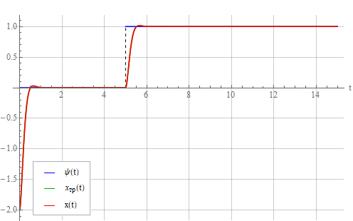
Now let’s give the control signal to the oscillator described by expression (6):
It can be seen that the oscillator behaves in accordance with the required law. Let's look at the control signal :
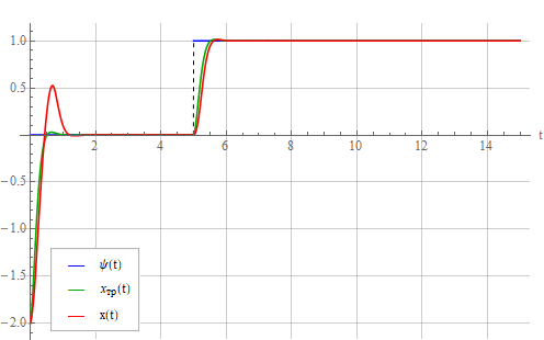
The figure shows a significant surge at the time of the transition process. In a real system, most likely, either the system will enter saturation (destruction), or in order to prevent this, we will have to limit the input signal. We take this into account by limiting the amplitude of the control action at the level 15. The control signal now looks like this:
and the oscillator output is like this:
The consequence of the signal limitation is a large transient error, which, depending on the desired properties of the system, can be quite significant. With an increase in the required time constant, transient emissions decrease. You need to be careful that the maximum control signal in the steady state (which on this graph starts from about the sixth second) is not limited, otherwise there will be an endless transient and the system will not work out the task. Regulator gain, i.e. control signal ratio at the regulator output determined by the parameters of the controlled system, namely the factor .
Now let’s feed the oscillator with such a linearly changing signal:
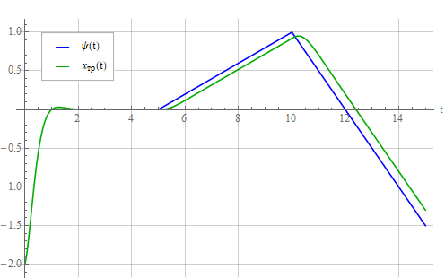
The reaction of the vibrational link:
and oscillator:
It is seen that a constant lag has appeared - a dynamic error, because the system is designed to track only a constant setting signal . In order to be able to track a linearly varying signal, it is necessary to evaluate the rate of its change and take it into account in the controller. To do this, we compose the required control law as follows:
Where - error tracking the master signal by the oscillator.
We also express the highest derivative from (7), substitute it into the equation of the control object (4) and get the control signal:
In the new structure of the regulator corresponding to expression (8), the rate of change of the set action . We look at the output of the system when a linearly varying setpoint is applied to the input:
Oscillator tracks the set signal .
But this is a completely synthetic example. In reality, there will be a system whose structure is probably not identified accurately enough - this time. We will also determine the system parameters with a certain error - these are two. Control includes phase variables that will have to be measured with some kind of noise are three. And the parameters of the system can float away over time, that is, a stationary system over a sufficiently long period of time can show non-stationarity. Although it’s more correct to say so - on a fairly short time interval, a non-stationary system may seem stationary. In this example, we assume that the system is identified with sufficient accuracy and its change in time is very insignificant. Then, for clarity, we rewrite the expression for controller (6) as follows:
Where - measured controlled value and its derivative; - identified natural frequency and non-linear attenuation coefficient, respectively.
Add a 10% error in the identification of the oscillator parameters by setting . Let's look at the result:
It can be seen from the figure that a static error appeared, which grows with an increase in the identification error and in steady state is independent of error . But the latter affects the deviation of the oscillator transient from that for the ideal oscillatory link. You can try to do the same as in the design of PID controllers ( Habr and not Habr ) - add the integral of the error to the control signal (without forgetting about the integral saturation once or twice ). But for now, we omit this question and consider expression (9), where it can be seen that the lower the natural frequency compared to the required time constant , the smaller the influence of the identification error of the same . Reduce from 0.125 to 0.05. Static error also decreased:
Now let’s try to compensate for the static error by adding the integral of the error to the controller (as in the PI controller). Expression (9) will turn into
Where - coefficient of the integral component; - current time.
The integral here is formally written as explaining the general idea, rather than the mathematical description of a specific algorithm, since in a real controller it is necessary to take measures to limit the accumulated error, otherwise problems with the transient can occur. Let us take a look at the reaction of the system under the action of the resulting regulator corresponding to expression (10):
It can be seen from the figure that the static error decreases over time, but the transient process is delayed. By analogy with the PID controller, you can try to add proportional and differentiating components. The result was as follows (the coefficients were not carefully chosen):
Naturally, the addition of the integral and differential components is no longer part of the inverse dynamics problem method, but implements a certain method for optimizing the transient process.
Let us analyze the effect of noise measurements of variables . Again, we feed a step to the system input and look at the output in the absence of any noise (there is still the same 10% identification error):
Now add to the measurements white Gaussian noises with zero expectation and equal variances passed through aperiodic links with time constants that simulate a measuring sensor + low-pass filter . One of the resulting noise implementations:
Now the system output also began to make noise:
as a result of a noisy control signal:
Take a look at the error working out the task:
Let's try to increase the time constants of the sensors and look at the system output again:
Significant fluctuations appeared - the result of the very unaccounted for small dynamic parameters [2] describing the sensors (their inertia). These dynamic parameters make noise filtering difficult, forcing to describe sensors with “large” time constants, which, generally speaking, cannot always give a positive result.
Control of a DC motor taking into account nonlinear viscous friction
This is a more real case of applying the inverse dynamics problem method. Consider the organization of control of a DC collector motor with excitation from permanent magnets (ala Chinese motors from toys). In principle, the topic of controlling such engines is well covered and does not cause any particular difficulties. The inverse dynamics problem method will be used by and large to compensate for non-linearity in the engine dynamics equation. We assume that the engine itself could be described by linear differential equations, but there is a significant influence of the nonlinear viscous friction of the shaft, proportional to the square of its rotation speed. The equation of the electromechanical system is as follows:
Where - angular velocity of rotation of the shaft; - moment of inertia of the entire rotating system (anchors with attached load); - a machine constant, defined for a specific engine design, relating magnetic flux and shaft rotation speed; - magnetic flux, which can roughly be considered constant for a particular motor design in the range of operating currents (but in the case of high currents non-linearly dependent on the winding current); - current through the armature winding; - coefficient of linear viscous friction; - coefficient of nonlinear viscous friction; - load moment; - inductance of the armature winding; - voltage applied to the winding; - coefficient of counter-EMF, constant for a specific engine design; - resistance of the armature winding.In principle, it would be sufficient to get along with only non-linear viscous friction, but it was decided to present the non-linear dependence of friction on the shaft rotation speed as a binomial for more generality.
We will try to make such a regulator by the method of the inverse problem of dynamics, so that the dynamics of the error in fulfilling the task in terms of speed by the engine corresponds to that for the vibrational link described by the expression
Where is the angular velocity of rotation of the motor shaft; - speed setting.
Equation (12) could be compiled using the error of working out the command as a dynamic variable :
but then the terms with derivatives of the setpoint would appear in the equation, as can be seen from the expression
This, in turn, would increase the fluctuation component of the error. And since we want the system to work out only a constant, abruptly changing set point (that is, considering its speed, acceleration and all subsequent derivatives to be zero), then we need to track the maximum error in position, not taking into account its derivatives, or, if it is easier to understand , with zero derivatives of the error, which would lead to expression (12).
To obtain an expression that finally describes the regulator, it is necessary to reduce the system of two first-order equations (11) to one second-order equation. To do this, we differentiate the first equation (11) in time (assuming that the load moment is unchanged):
and substitute into it the expression from the second equation of system (11) , which gives a second-order equation
Substituting into expression (13) obtained from (12) we can find the required control to implement the desired law of motion (12):
We apply to the inputs of two engines, one of which is supplemented by a regulator implemented according to the principle of the inverse dynamic problem, a step with a unit amplitude in accordance with the following scheme:
and see the dependence of the rotational speed of the motor shafts on time:
Reaction to a step with an amplitude of 10 volts:
From the figures, a nonlinear dependence of the oscillation index of the initial system on the amplitude of the input signal is visible.
Now compare two engines with PID controllers, the structural diagram of which is shown in the following figure:
Frequencies of rotation of shaft of engines:
and larger:
It can be seen from the figures that, thanks to the PID controller constructed using the inverse dynamic problem method, the system response to the step-by-step control signal was accelerated, which could not be achieved using the conventional PID controller due to the non-linearity in the control object. However, the use of variable coefficients of the PID controller would probably solve this problem better and make the system more robust. But this is a completely different story.
Conclusion
The article considered a method that allows you to build a controller for controlling non-linear systems, which was shown by examples of controls of the Van der Pol oscillator and a DC motor.
The main advantages of this method include:
- ease of implementation of the required control law (analytically);
- the ability to control non-linear systems;
- the ability to control non-stationary systems.
However, this method also has a number of significant disadvantages :
- the need to know the entire state vector of the managed system (which may require differentiation, filtering);
- the need for sufficiently accurate identification of the parameters of the controlled system, which can reduce robustness;
- the need to study the system for instability resulting from the combined action of small dynamic parameters (filters, sensors) not included in the model.
In general, this is a rather interesting method, but by comparing its implementation for controlling a DC motor (using a PID controller) with a motor controlled only by a PID controller, it became clear that significant buns could not be obtained from it. But the structure of the control device is much more complicated, forcing, among other things, to struggle with differentiation noises on the one hand, and preventing the stability boundary from reaching the other hand. Perhaps it is with this that a small number of works on this topic are connected. One of the possible applications of the method of the inverse problem of dynamics can be the construction of reference (ideal) trajectories of systems for comparison with trajectories corresponding to various controllers, for example, linear or linearized.
Used Books:
1. Kim D.P. Theory of automatic control. T.2. Multidimensional, nonlinear, optimal and adaptive systems: Textbook. allowance.- M .: FIZMATLIT, 2004 .-- 464 p.
2. Boychuk L.M. The method of structural synthesis of nonlinear automatic control systems. M., "Energy", 1971.
3. Non-stationary automatic control systems: analysis, synthesis and optimization / Ed. K.A. Pupkova and N.D. Egupova. - M .: Publishing house of MGTU im. N.E. Bauman, 2007 .-- 632 p.
All Articles