How to color polynomials correctly

Polynomials are not just exercises in abstract matters. They are great for spotting structures in unexpected places.

In 2015, a former poet who became a mathematician, Jun Ho helped solve the problem formulated about 50 years ago. It was associated with complex mathematical objects, " matroids ", and graphs (combinations of points and segments). And it was also connected with polynomials - expressions familiar to us from the lessons of mathematics, consisting of the sum of variables raised to various degrees.



At some point in school, you probably went through the opening of brackets in polynomials. For example, you may remember that x ² + 2xy + y ² = (x + y) ² . A convenient algebraic trick, but where can it come in handy? It turns out that polynomials perfectly help to reveal hidden structures - and Ho actively used this fact in his proof. Here is a simple riddle illustrating this.



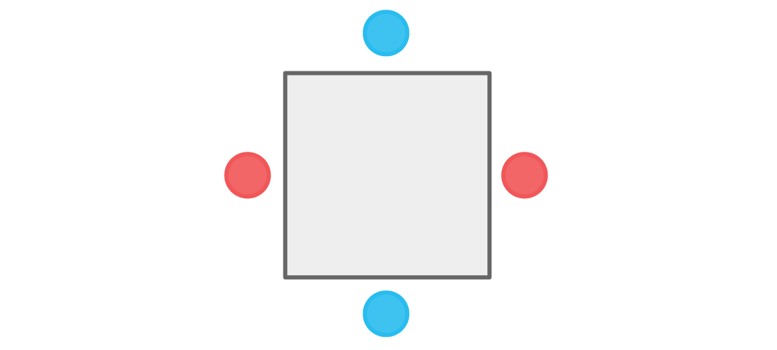
Suppose we need to seat two teams of players at a square table. To prevent fraud, you need to make sure that players do not sit next to other players on their team. How many seating methods are there?



Let's start with the seating of the red and blue team. Suppose a red player sits at the top of the chart:







There are two places near the top place - right and left - and to satisfy the rule, these places must be occupied by blue players.







The space below is adjacent to the two blue ones, so the red player must sit there.







None of the players are sitting next to a member of their team, and our condition is met.



We could also start with the blue player at the top. Similar considerations lead to the following arrangement:







And again, no player sits next to other members of his team. Our condition is fulfilled, and such a seating arrangement is acceptable. In fact, there are exactly two such seating arrangements. As soon as we choose the color of the top spot, all the rest are fully defined.



There is a way to find out that there are only two possible seating arrangements without drawing all of these diagrams. Let's start from the top: we have two options, red and blue. After this choice, there remains one option (a different color) for the left and right seats. And for the lower seat there is only one option left - the color with which we started. Using the “fundamental principle of calculation”, we know that the total number of possibilities is the result of multiplying the number of possibilities for each of the options. This gives us 2 × 1 × 1 × 1 = 2 seedlings, as we determined from our diagrams.



Now add the third command with the third color. Imagine that we have red, blue, and yellow players. How many seating arrangements can be made, provided that the neighboring places must be of different colors? To display all the possibilities, you have to draw a whole wagon of diagrams, so let's try to do the calculations instead.



For the top spot, we now have a choice of three colors. After this choice, we can choose any of the two remaining colors for the left and right places.



What will be below the square? There is a temptation to say that for the last seat there will be only one option, since it is next to both the left and right seats. But do you feel flawed in this logic?







Indeed, if the left and right places have different colors, then for the bottom place there will be only one option. If on the left, for example, it is blue and on the right is red, then the bottom must be yellow. But what if the left and right colors are the same? In this case, for the bottom place there will be a choice of two options. This last choice depends on the previous ones, which complicates our calculations.



We have to consider two different cases: when the colors on the left and on the right coincide, and when they differ.



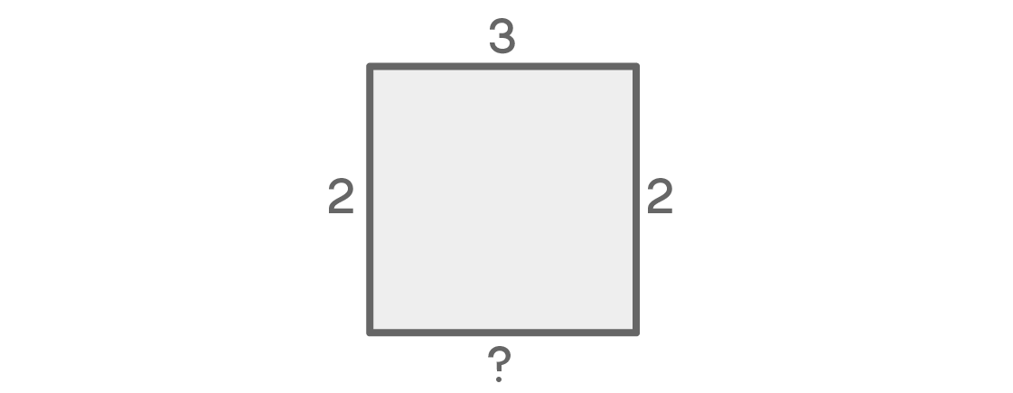
If the colors on the left and right coincide, the number of possibilities for each of the places looks like this:







For the upper seat, we have three options. There are two left for the right. Since we assume that the left and right places have the same color, we only have one option for the left place: the same color as the right. Finally, since the color is the same on the left and right, we can choose either of the two remaining colors for the lower seat. As a result, we get 3 × 2 × 1 × 2 = 12 possible seating arrangements.



Now let's look at those possibilities when the colors on the right and left are different:







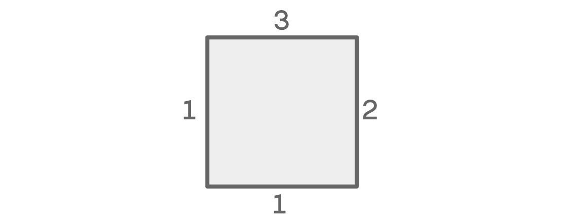
We again have three options for the top and two for the right place. The left place again has one option, but for a different reason: it cannot be the same as the top, neighboring one, and cannot be the same as the right, according to our condition. And, since the colors on the right and left are different, there is only one option left for the bottom place (the same as the top). This case gives 3 × 2 × 1 × 1 = 6 possible arrangements.



Since these two options cover all the possibilities, we add them up and get 12 + 6 = 18 possible seating arrangements.



Adding a third color complicated our task, but our hard work will be rewarded. Now we can use this strategy for 4, 5 or any number q of different colors.



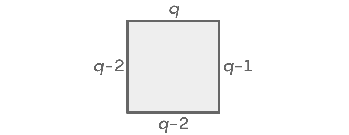
Regardless of the number of colors, we will always have two cases: left and right will be either the same or different colors. Suppose we have a choice of q colors. Here is a chart showing the number of options for each side, in the case where the right and left colors are the same:







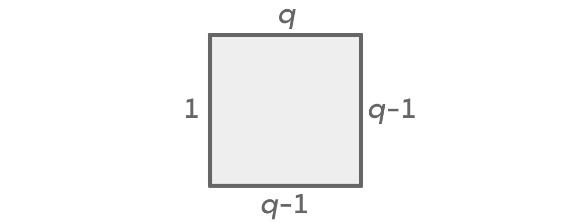
First we have q colors for the upper seat, and q-1 for the right. Since we assumed that the colors on the left and right are the same, we have only one option for the left color. This leaves q-1 options for the bottom place, because it can be of any color except the one we chose for the left and right places. The fundamental principle of calculation gives us q × (q - 1) × 1 × (q - 1) = q (q - 1) ² possible solutions.



If the left and right places are colored differently, then we can calculate the possibilities like this:







Once again, we have q options for the top and q-1 for the right places. There cannot be the same color on the left that is selected for the top and right places, so there are q-2 options. There can be any color below, except for the two that we used left and right, which again gives q-2 options. We get in the sum q × (q - 1) × (q - 2) × (q - 2) = q (q - 1) (q - 2) ² possible seating arrangements. Since these two situations cover all the options, we, as before, add them up and get the total number of possible arrangements: q (q - 1) ² + q (q - 1) (q - 2) ² .



Such an expression may seem like a strange answer to the question “How many different seating arrangements of different teams at the square table, such that two members of the same team will not sit side by side?” However, this polynomial contains a lot of information about our problem. He not only gives us a quantitative answer, but also reveals the structure of our task.



Such a polynomial is called a “ chromatic polynomial ” because it answers the question: how many methods exist for coloring the vertices of a network (or graph) such that any pair of neighboring vertices has different colors?



Initially, our problem was related to the seating around the table, but we can easily turn it into a question about coloring the vertices of the graph. Instead of people at the table:







we imagine them in the form of peaks connected by edges in the case when they are sitting next to:







Now, any coloring of the vertices of the graph can be represented as the seating of people around the square, where “sit next to” at the table means “have a common edge” on the graph.



Now, having reformulated our problem in the form of a graph, we return to the chromatic polynomial. We call it P (q).



P (q) = q (q - 1) ² + q (q - 1) (q - 2) ²



A remarkable property of this polynomial is that it answers the coloring question for any possible number of colors. For example, to answer a question with three colors, we put q = 3, and we get:



P (3) = 3 (3 - 1) ² + 3 (3 - 1) (3 - 2) ² = 3 × 2 ² + 3 × 2 × 1 ² = 12 + 6 = 18



This is the answer we received in the case of three teams. And if we put q = 2:



P (2) = 2 (2 - 1) ² + 2 (2 - 1) (2 - 2) ² = 2 × 1 ² + 2 × 1 × 0 ² = 2 + 0 = 2



Sounds familiar? This is the answer to our first riddle, with two teams. We can find answers for four, five or even 10 different teams, simply substituting the desired value for q: P (4) = 84, P (5) = 260 and P (10) = 6 570. The chromatic polynomial caught some fundamental structure of the problem summarizing our counting strategy.



We can reveal more details of the structure by performing algebraic operations on our polynomial P (q) = q (q - 1) ² + q (q - 1) (q - 2) ² :



= q (q − 1) (q − 1) + q (q − 1) (q − 2) ²

= q (q − 1) ((q − 1) + (q − 2) ² )

= q (q − 1) (q − 1 + q ² −4q + 4)

= q (q − 1) (q ² −3q + 3)



We extracted the factor q (q - 1) from each part of the sum and combined similar terms, reducing the polynomial to a factorized form. And in this form, the polynomial can tell us about the structure with the help of its “roots”.



The roots of a polynomial are input values ​​at which it becomes equal to zero at the output. In the factorized form, it is easier to find the roots: since the polynomial is expressed as multiplied parts, any value at which one of the factors is equal to zero resets the whole product.



For example, our polynomial P (q) = q (q - 1) (q ² - 3q + 3) has a factor (q - 1). If we take q = 1, this factor becomes equal to zero, like the whole result of multiplication. That is, P (1) = 1 (1 - 1) (1 ² - 3 × 1 + 3) = 1 × 0 × 1 = 0. Similarly, P (0) = 0 × (–1) × 3 = 0 Therefore, q = 1 and q = 0 are the roots of our polynomial. (You may be interested in the factor (q ² - 3q + 3). Since it is not equal to zero for any real q, it does not give new roots to our chromatic polynomial).



These roots make sense within the framework of our graph. If we have a choice of the same color, each vertex must be the same color. It is not possible to color the graph so that all adjacent vertices have different colors. This is precisely what means that q = 1 is the root of our chromatic polynomial. If P (1) = 0, then there are exactly zero ways to color the graph so that the neighboring vertices are not the same colors. The same is true for the version with zero number of colors, P (0) = 0. The roots of our chromatic polynomial tell us about the structure of our graph.



The ability to see structure through algebra becomes even more obvious if we consider other graphs. Let's look at a triangular graph:







How many ways are there to color this graph q with colors so that the neighboring vertices are not the same colors?



As usual, for the first two neighboring vertices there are q and q-1 options. And since the last vertex is adjacent to the first two, it should differ in color from both of them, which leaves us with q-2 options. This gives us the chromatic polynomial for this triangular graph: P (q) = q (q - 1) (q - 2).



In this form of factorization, this chromatic polynomial tells us something interesting: it has a root q = 2. And if P (2) = 0, it should be impossible to color this graph with two colors so that it does not have two adjacent vertices of the same color. Is it so?



Imagine that we are walking in a circle in this triangle, coloring the peaks along the way. If we have only two colors, we need to alternate them after each vertex: if the first is red, then the second will be blue, which means that the third should again be red. But the first and third peaks are adjacent, and they cannot be red both. Two colors are not enough, as the polynomial predicted.



Using a similar argument with alternation, we can come to a significant generalization: the chromatic polynomial of any closed loop with an odd number of vertices must have a root equal to 2. Since if you alternate two colors and move along a loop of odd length, the first and last colored vertices will be the same color . But just as this is a loop, they will be adjacent. Coloring is not possible.



For example, we can use various techniques to determine that for a loop with five vertices the chromatic polynomial looks like this: P (q) = q ⁵ - 5q ⁴ + 10q ³ - 10q ² + 4q. Factoring this out, we get P (q) = q (q - 1) (q - 2) (q2 - 2q + 2). As expected, it turns out that q = 2 is the root, and P (2) = 0. Interestingly, as soon as we find this connection between the graphs and their polynomials, ideas begin to work in both directions. Polynomials can tell us information about the structure of graphs, and graphs can tell us about the structure of polynomials.



It was the search for structure that led June Ho to prove Reed's 40-year hypothesis regarding chromatic polynomials. The hypothesis states that if we enumerate the coefficients of the chromatic polynomial in order, ignoring their signs, then the following condition will be fulfilled: the square of any coefficient must be at least the product of two neighboring ones. For example, in the chromatic polynomial for our loop of five vertices, P (q) = q ⁵ - 5q ⁴ + 10q ³ - 10q ² + 4q, we see that 5 ² ≥ 1 × 10, 10 ² ≥ 5 × 10 and 10 ² ≥ 10 × 4. From this, for example, it follows that not every polynomial can be chromatic: chromatic polynomials associated with graphs have a deeper structure. Moreover, the connection between these polynomials and other domains allowed Ho and his co-authors to answer a much broader question related to the Roth hypothesis, several years after the proof of the Reed hypothesis.



Perhaps the polynomials are best known for their worst form — as abstract exercises in the formal manipulation of algebraic expressions. But the polynomials and their properties - roots, coefficients, various forms - help to reveal structures in unexpected places, creating connections with algebra in everything that surrounds us.

Exercises

1. A complete graph is a graph, each pair of vertices of which is connected by an edge. Find the chromatic polynomial of a complete graph of five vertices.





2. Find the chromatic polynomial for the next graph (use information about the chromatic polynomials of simpler graphs).









3. A graph is called two-sided if its vertices can be divided into two groups, A and B, so that vertices from A are adjacent only to vertices B, and vertices B are adjacent only to vertices from A. Suppose graph G has a chromatic polynomial P (q). What property P (q) allows you to conclude that the graph G is two-sided?