Converting Polygonal Models to Boundary Representation: Algorithm and Code Examples
In most design systems (CAD), the main representation of the simulated object is the boundary representation of geometry or B-rep (Boundary representation). But increasingly, CAD users have to deal with polygon models, for example, obtained as a result of 3D scanning or borrowed from online catalogs.
To make them suitable for further work, you need to convert the polygon mesh into a B-rep model. And this is not easy at all.
We have developed the C3D B-Shaper software component, which is integrated into the design system and converts polygonal models into a boundary representation. In this post we will show the conversion algorithm and implementation examples in C ++.

What is the main problem of polygonal models in terms of CAD? Traditional tools cannot be applied to them - to perform Boolean operations, to construct chamfers and fillets, to obtain projections and sections. If using the B-rep model to build its polygonal representation is quite easy (this is done using triangulation), then the inverse transformation is much more difficult. A number of problems arise - the recognition of surfaces of various types (including free-form surfaces), the presence of noise, which are characteristic, for example, of 3D scanning results.
In the new SDK, we implemented a three-stage mechanism for converting the polygonal model into B-rep: segmentation, surface reconstruction, construction of the B-rep model. In general, the process is assumed to be iterative: if for some reason the user is not satisfied with the result, then he can make the necessary corrective changes at the stages of segmentation and reconstruction of surfaces.
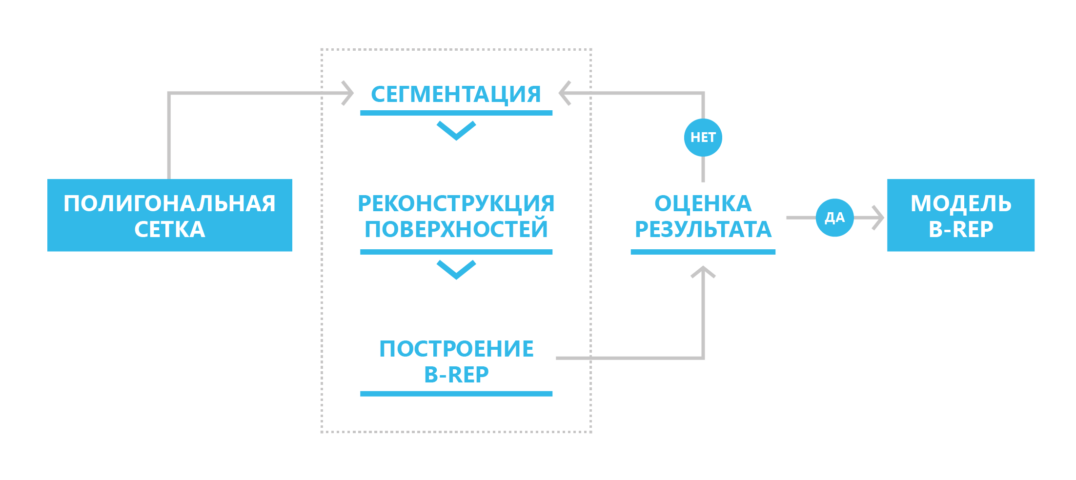
The scheme for converting a polygonal representation to a boundary
Before initiating the conversion process to B-rep, it is necessary, in some cases, to improve the quality of the original polygonal mesh: coordinate the normal directions at neighboring polygons, eliminate “holes”, apply smoothing algorithms in the presence of noise in the original mesh.
At the first stage, the initial set of mesh polygons is classified into subsets (segments). Information about the normals at the vertices of the mesh allows first-order segmentation and thereby ensures the initial mesh partition, as well as classify flat or strongly curved areas.
The initial meshing is based on the definition of so-called “sharp” edges — such edges between two triangular polygons whose angle between the average normals exceeds a certain predetermined value.
Second-order segmentation analyzes the grid in accordance with its main curvatures, which provides a sufficient foundation for the classification of elementary surfaces. In calculating the curvatures at the vertices of the grid, we used the results of Mayer (Mark Meyer, Mathieu Desbrun, Peter Schroder, and Alan H. Barr, Discrete Differential-Geometry Operators for Triangulated 2-Manifolds, Visualization and Mathematics III, 2003) to determine the discrete differential operator for triangulated regions: for each vertex of the original mesh, we consider a set of neighboring vertices associated with a given vertex through an edge. Then, a discrete operator K is calculated for a given vertex, based on which the average normal, average K H, and Gaussian K G curvature at the vertex of the grid are determined.
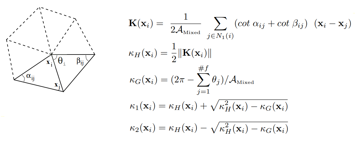
On the definition of a discrete differential operator for triangulated domains
Thus, the curvature tensor for each vertex of the grid is calculated, the eigenvalues of which are the desired main curvatures K 1 and K 2 , and the eigenvectors are the main directions of the curvature change.
Next, the mesh vertices are classified according to the values of the main curvatures K 1 and K 2 calculated in them. The vertex classification algorithm is based on the k-means method, i.e., on minimizing the total quadratic deviation of cluster points from the centers of these clusters. As a result, at the output of the algorithm, each vertex of the grid is associated with a certain cluster and a pair of curvatures (cluster center) (L. Guillaume, “Curvature Tensor Based Triangle Mesh Segmentation with Boundary Rectification”, Proceedings Computer Graphics International (CGI), 2004).
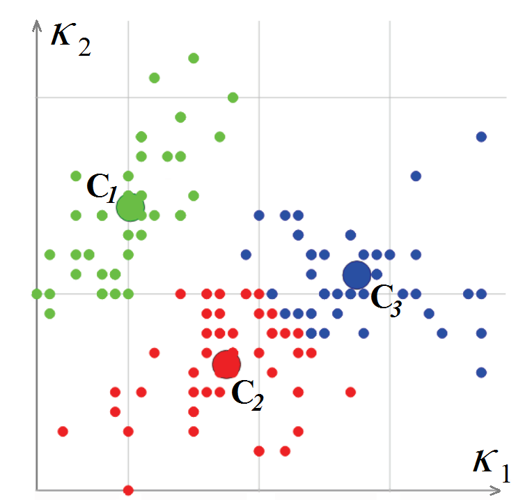
Classification of the vertices of a polygonal mesh in the space of curvatures
After classifying the vertices of the polygonal mesh, it is necessary to classify the polygons. At the beginning of this procedure, a triangular polygon is selected for which the curvature can be considered completely defined (all three vertices belong to one cluster or two vertices lie on a sharp edge). This polygon is declared a new segment, and the recursive procedure for expanding the segment starts from it: for each triangular polygon, the polygons adjacent to it are considered, provided that the edge between them is not “sharp”.
If the vertex of a neighboring polygon, opposite the common edge, lies on a sharp edge or belongs to the same cluster, then this polygon is added to the segment. The process is repeated until all polygons of this grid are viewed. Here's what the implemented mesh segmentation mechanism looks like.
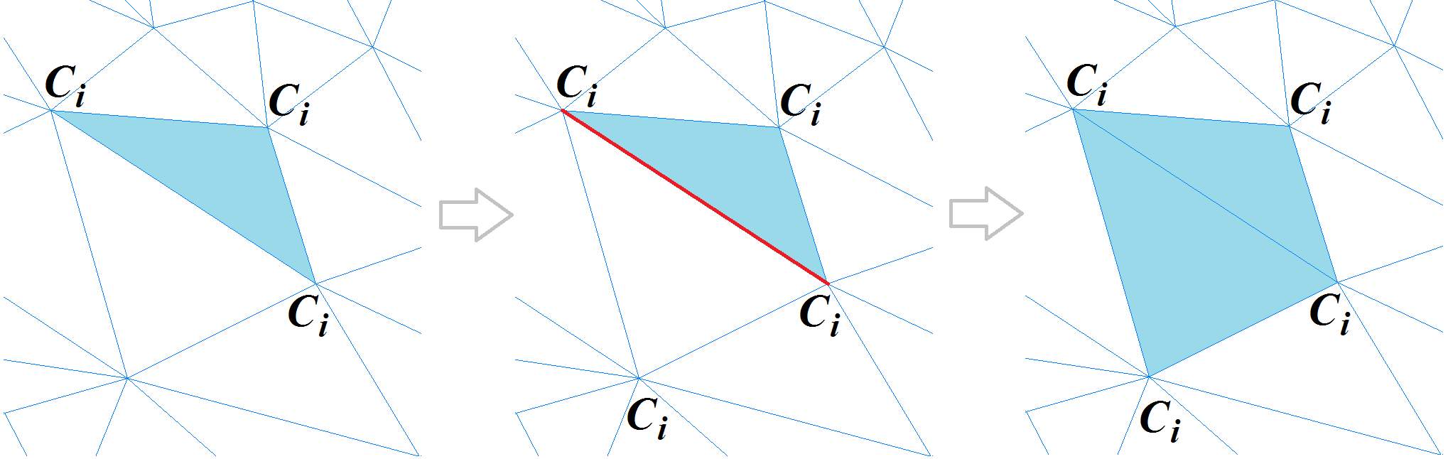
Polygon mesh segmentation mechanism
At the end of the segment formation procedure, a special algorithm for stitching adjacent segments is performed to eliminate excessive segmentation of the mesh in question.
At the second stage, each of the segments must be associated with a certain surface approximating its shape with a given accuracy. First of all, the values of the main curvatures for this segment determine the possibility of describing the shape of the segment by an elementary surface:
If none of the elementary surfaces is suitable for describing a segment, the algorithm will try to recognize the extrusion or rotation surface. Ultimately, if it was not possible to select an analytical surface to describe the shape of the segment, a NURBS surface will be built for it.
Elementary surfaces are constructed using methods of fitting simple geometric objects into a set of points. So, the least squares method is used to fit the circle and sphere, and the principal component method is used to fit the plane. Each reconstructed surface is checked for compliance with a segment by a given recognition accuracy.
For clarity, we painted the recognized surfaces in different colors: planes - blue, cylinders - red, spheres - green, cones - yellow, tori - purple.
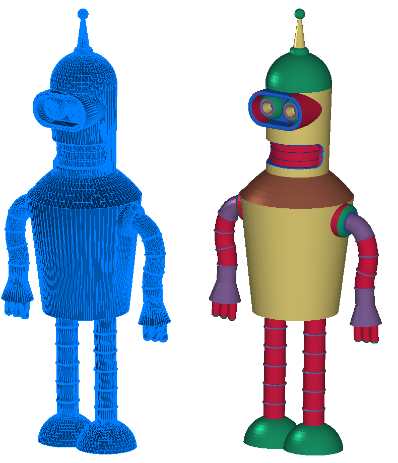
Original polygon mesh (left) and segmented mesh (right) with surfaces recognized on segments
The final stage of the transformation is the construction of a B-rep model based on segmentation of the recognized surfaces. In this approach, a graph of adjacent regions is constructed on the basis of segmented regions, which reflects the topology of the model and serves as the basis for constructing the final B-rep model.
Unlike the previous stages of conversion, the B-rep assembly is carried out in a fully automatic mode: the intersection lines of neighboring reconstructed surfaces are found, the edges of the faces are built on them, the faces themselves and, finally, the B-rep shell is assembled.

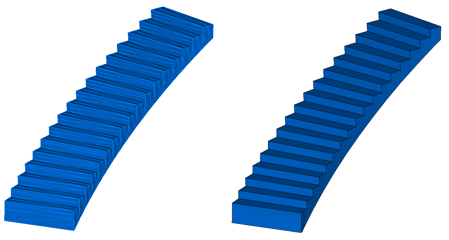
Original polygon mesh (left) and B-rep model (right)
However, it is not always possible to construct a topologically correct shell. As an example of such a situation, suppose that during the reconstruction of surfaces we have two surfaces - a cylinder and a plane, and their position in space is close to tangent. Due to errors in the reconstruction of the surfaces of their intersection, there may not be any at all. In such cases, the shell may be built with some defects that the user can fix by properly adjusting the surface parameters.
Today, there are several main sources of models in the polygonal representation:
Polygonal models from these sources can be divided into two groups: the first includes models that are triangulations of B-rep objects, and the second - all the others. The characteristic differences of the first group are the absence of noise in the polygonal mesh and the predominance of analytically defined surfaces. Thus, the conversion to the B-rep models from the first group will take place either in fully automatic mode or with minimal user intervention.
Polygonal grids of the models of the second group imply a denser interactive interaction with the user. Therefore, initially we laid down two operating modes in the C3D B-Shaper - fully automatic and interactive.
The choice of a particular mode also depends on the purpose of the transformation: in some cases, the topological connectivity of the elements of the resulting shell, as well as its correctness, can be neglected. Such an approach is acceptable, for example, to optimize rendering in a BIM application, when the user can add arbitrary interior items to the current model of the room. On the other hand, for reverse engineering tasks it is necessary to obtain the most accurate copy of the original model, for example, to preserve the alignment of the cylinders with a given accuracy, to ensure the tangent location of a pair of surfaces and, as a result, to obtain the correct topology of the model - in this case, you can not do without user intervention in conversion process.
The C3D B-Shaper automatic conversion interface is represented by the following functions, which accept the input grid and conversion settings as input:
The conversion settings include the recognition accuracy value, i.e. the maximum allowable distance of the vertices of the polygonal mesh within the boundaries of this segment to the recognized surface. This accuracy can be absolute or relative: when using relative accuracy, the deviation of the faces of the body from the grid is checked with respect to the size of the model.
Also, the user has the option of switching recognition modes, which allows you to control the types of surfaces during reconstruction.
Advanced capabilities for managing segmentation and surface recognition processes are provided by the MbMeshProcessor class interface:
For example, to correct the results of automatic segmentation, tools are provided for combining segments, separating them, etc. The user can enter a surface of a given type in a segment, as well as change the parameters for an already recognized surface.
In July, we released the first version of the component and are now continuing to develop in several areas: automatic segmentation algorithms, segmentation editing tools, building free-form surfaces (NURBS) based on a segment, and improving the build quality of B-rep shells.
Interested developers can test the C3D B-Shaper. The component is provided free of charge for three months upon request on our website.
To make them suitable for further work, you need to convert the polygon mesh into a B-rep model. And this is not easy at all.
We have developed the C3D B-Shaper software component, which is integrated into the design system and converts polygonal models into a boundary representation. In this post we will show the conversion algorithm and implementation examples in C ++.
What is the main problem of polygonal models in terms of CAD? Traditional tools cannot be applied to them - to perform Boolean operations, to construct chamfers and fillets, to obtain projections and sections. If using the B-rep model to build its polygonal representation is quite easy (this is done using triangulation), then the inverse transformation is much more difficult. A number of problems arise - the recognition of surfaces of various types (including free-form surfaces), the presence of noise, which are characteristic, for example, of 3D scanning results.
In the new SDK, we implemented a three-stage mechanism for converting the polygonal model into B-rep: segmentation, surface reconstruction, construction of the B-rep model. In general, the process is assumed to be iterative: if for some reason the user is not satisfied with the result, then he can make the necessary corrective changes at the stages of segmentation and reconstruction of surfaces.
The scheme for converting a polygonal representation to a boundary
Before initiating the conversion process to B-rep, it is necessary, in some cases, to improve the quality of the original polygonal mesh: coordinate the normal directions at neighboring polygons, eliminate “holes”, apply smoothing algorithms in the presence of noise in the original mesh.
Polygon segmentation
At the first stage, the initial set of mesh polygons is classified into subsets (segments). Information about the normals at the vertices of the mesh allows first-order segmentation and thereby ensures the initial mesh partition, as well as classify flat or strongly curved areas.
The initial meshing is based on the definition of so-called “sharp” edges — such edges between two triangular polygons whose angle between the average normals exceeds a certain predetermined value.
Second-order segmentation analyzes the grid in accordance with its main curvatures, which provides a sufficient foundation for the classification of elementary surfaces. In calculating the curvatures at the vertices of the grid, we used the results of Mayer (Mark Meyer, Mathieu Desbrun, Peter Schroder, and Alan H. Barr, Discrete Differential-Geometry Operators for Triangulated 2-Manifolds, Visualization and Mathematics III, 2003) to determine the discrete differential operator for triangulated regions: for each vertex of the original mesh, we consider a set of neighboring vertices associated with a given vertex through an edge. Then, a discrete operator K is calculated for a given vertex, based on which the average normal, average K H, and Gaussian K G curvature at the vertex of the grid are determined.
On the definition of a discrete differential operator for triangulated domains
Thus, the curvature tensor for each vertex of the grid is calculated, the eigenvalues of which are the desired main curvatures K 1 and K 2 , and the eigenvectors are the main directions of the curvature change.
Next, the mesh vertices are classified according to the values of the main curvatures K 1 and K 2 calculated in them. The vertex classification algorithm is based on the k-means method, i.e., on minimizing the total quadratic deviation of cluster points from the centers of these clusters. As a result, at the output of the algorithm, each vertex of the grid is associated with a certain cluster and a pair of curvatures (cluster center) (L. Guillaume, “Curvature Tensor Based Triangle Mesh Segmentation with Boundary Rectification”, Proceedings Computer Graphics International (CGI), 2004).
Classification of the vertices of a polygonal mesh in the space of curvatures
After classifying the vertices of the polygonal mesh, it is necessary to classify the polygons. At the beginning of this procedure, a triangular polygon is selected for which the curvature can be considered completely defined (all three vertices belong to one cluster or two vertices lie on a sharp edge). This polygon is declared a new segment, and the recursive procedure for expanding the segment starts from it: for each triangular polygon, the polygons adjacent to it are considered, provided that the edge between them is not “sharp”.
If the vertex of a neighboring polygon, opposite the common edge, lies on a sharp edge or belongs to the same cluster, then this polygon is added to the segment. The process is repeated until all polygons of this grid are viewed. Here's what the implemented mesh segmentation mechanism looks like.
Polygon mesh segmentation mechanism
At the end of the segment formation procedure, a special algorithm for stitching adjacent segments is performed to eliminate excessive segmentation of the mesh in question.
Surface recognition
At the second stage, each of the segments must be associated with a certain surface approximating its shape with a given accuracy. First of all, the values of the main curvatures for this segment determine the possibility of describing the shape of the segment by an elementary surface:
- plane: k 1 = k 2 = 0
- sphere: k 1 = k 2 = K > 0
- cylinder: k 1 = K > 0, k 2 = 0
- cone: k 1 ∈ [ a , b ], k 2 = 0
- torus: k 1 = K , k 2 ∈ [ a , b ]
If none of the elementary surfaces is suitable for describing a segment, the algorithm will try to recognize the extrusion or rotation surface. Ultimately, if it was not possible to select an analytical surface to describe the shape of the segment, a NURBS surface will be built for it.
Elementary surfaces are constructed using methods of fitting simple geometric objects into a set of points. So, the least squares method is used to fit the circle and sphere, and the principal component method is used to fit the plane. Each reconstructed surface is checked for compliance with a segment by a given recognition accuracy.
For clarity, we painted the recognized surfaces in different colors: planes - blue, cylinders - red, spheres - green, cones - yellow, tori - purple.
Original polygon mesh (left) and segmented mesh (right) with surfaces recognized on segments
Building a B-rep Model
The final stage of the transformation is the construction of a B-rep model based on segmentation of the recognized surfaces. In this approach, a graph of adjacent regions is constructed on the basis of segmented regions, which reflects the topology of the model and serves as the basis for constructing the final B-rep model.
Unlike the previous stages of conversion, the B-rep assembly is carried out in a fully automatic mode: the intersection lines of neighboring reconstructed surfaces are found, the edges of the faces are built on them, the faces themselves and, finally, the B-rep shell is assembled.
Original polygon mesh (left) and B-rep model (right)
However, it is not always possible to construct a topologically correct shell. As an example of such a situation, suppose that during the reconstruction of surfaces we have two surfaces - a cylinder and a plane, and their position in space is close to tangent. Due to errors in the reconstruction of the surfaces of their intersection, there may not be any at all. In such cases, the shell may be built with some defects that the user can fix by properly adjusting the surface parameters.
Types of polygonal models and the choice of conversion mode
Today, there are several main sources of models in the polygonal representation:
- Online catalogs, databases of 3D models in polygon format (STL, VRML, OBJ), for example 3D Warehouse, Cults 3D, etc.
- 3D scan results
- results of topological model optimization by CAE-algorithms.
Polygonal models from these sources can be divided into two groups: the first includes models that are triangulations of B-rep objects, and the second - all the others. The characteristic differences of the first group are the absence of noise in the polygonal mesh and the predominance of analytically defined surfaces. Thus, the conversion to the B-rep models from the first group will take place either in fully automatic mode or with minimal user intervention.
Polygonal grids of the models of the second group imply a denser interactive interaction with the user. Therefore, initially we laid down two operating modes in the C3D B-Shaper - fully automatic and interactive.
The choice of a particular mode also depends on the purpose of the transformation: in some cases, the topological connectivity of the elements of the resulting shell, as well as its correctness, can be neglected. Such an approach is acceptable, for example, to optimize rendering in a BIM application, when the user can add arbitrary interior items to the current model of the room. On the other hand, for reverse engineering tasks it is necessary to obtain the most accurate copy of the original model, for example, to preserve the alignment of the cylinders with a given accuracy, to ensure the tangent location of a pair of surfaces and, as a result, to obtain the correct topology of the model - in this case, you can not do without user intervention in conversion process.
The C3D B-Shaper automatic conversion interface is represented by the following functions, which accept the input grid and conversion settings as input:
MbResultType ConvertMeshToShell( MbMesh & mesh, MbFaceShell *& shell, const MbMeshProcessorValues & params ); MbResultType ConvertCollectionToShell( MbCollection & collection, MbFaceShell *& shell, const MbMeshProcessorValues & params );
The conversion settings include the recognition accuracy value, i.e. the maximum allowable distance of the vertices of the polygonal mesh within the boundaries of this segment to the recognized surface. This accuracy can be absolute or relative: when using relative accuracy, the deviation of the faces of the body from the grid is checked with respect to the size of the model.
Also, the user has the option of switching recognition modes, which allows you to control the types of surfaces during reconstruction.
Advanced capabilities for managing segmentation and surface recognition processes are provided by the MbMeshProcessor class interface:
class MbMeshProcessor { .. public: // “” . void SetUseMeshSmoothing( bool useSmoothing ); // . const MbCollection & GetSegmentedMesh(); MbResultType SegmentMesh( bool createSurfaces = true ); void ResetSegmentation(); void UniteSegments( size_t firstSegmentIdx, size_t secondSegmentIdx ); MbResultType SegmentMeshBySeparators( const std::vector<std::vector<uint>> & sep ); // . void FitSurfaceToSegment( size_t idxSegment ); void FitSurfaceToSegment( size_t idxSegment, MbeSpaceType surfaceType ); const MbSurface * GetSegmentSurface( size_t idxSegment ) const; // B-rep . MbResultType CreateBRepShell( MbFaceShell *& pShell ); .. }
For example, to correct the results of automatic segmentation, tools are provided for combining segments, separating them, etc. The user can enter a surface of a given type in a segment, as well as change the parameters for an already recognized surface.
What is happening now
In July, we released the first version of the component and are now continuing to develop in several areas: automatic segmentation algorithms, segmentation editing tools, building free-form surfaces (NURBS) based on a segment, and improving the build quality of B-rep shells.
Interested developers can test the C3D B-Shaper. The component is provided free of charge for three months upon request on our website.
All Articles