Study of modal control magnetic levitation system

This material was created in view of the past defense of the final qualification work of the bachelor, taking into account some comments on the control object. The material is created as an initial reserve for a possible master's thesis on the same subject.

Modern magnetic levitation systems are becoming more and more widely used: high-speed passenger trains, isolation of vibration-sensitive mechanisms, magnetic bearings, levitation of molten metal in induction furnaces, as well as levitation of metal billets. Recently, the effect of magnetic levitation is also used in household appliances.

Perhaps the most significant application was found in trains with a levitation system on superconductors. And this is due to such advantages as greater reliability (due to the lack of friction), relatively low power consumption, and the ability to develop high speed.

However, due to the nonlinear equations of motion of the object that describe its dynamics, it is difficult to reproduce the process of controlling the object. It will be about the position (distance) of the object relative to the zero mark.

In short, magnetic levitation is a stable position of an object at a certain distance in a gravitational field, when, as a rule, the acceleration of gravity is compensated by the acceleration of the object, which is created by a magnetic field. In this case, lifting force arises.

Magnetic levitation is realized using diamagnetics, eddy current systems and superconductors, as well as using servomechanisms.

In the current article (under the cut), we will consider modal control for a linearized system of magnetic levitation, as well as the implementation of modal control for a nonlinear model of the system.

Mathematical model

Consider a simple magnetic levitation scheme.

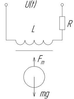
This diagram shows an electromagnet that interacts with the magnetic field of the control object, which is a ball-permanent magnet. Through a change in the force of attraction of the electromagnet, the levitation effect will be achieved.

In the final work, an object of the second order was considered, where one important component, the current in the coil, was not included in the state vector. This time this component will be introduced.

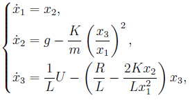
Where $$$x_1$ - position of the object;

$$$x_2$ - the rate of change in the position of the object;

$$$g$ - acceleration of gravity;

$$$K$ Is a constant;

$$$m$ - mass of the ball object;

$$$x_3$ - current in the coil;

$$$L$ - coil inductance;

$$$U$ - input voltage;

$$$R$ - active resistance of the coil.

The values ​​of some of the above variables are summarized in a table.

To obtain a linear model, one should linearize the system of equations.

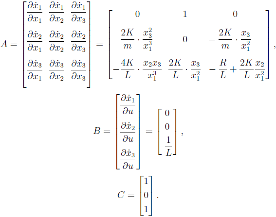
Matrix view $$$C$ can be justified by the fact that such state vector variables as position ( $$$x_1$ ) and current ( $$$x_3$ )

In this form, the resulting matrices are still not suitable for modeling. To do this, we set the initial conditions.

$$

$$x_1 ^ {\ left \ {0 \ right \}} = 0.005, ~ x_2 ^ {\ left \ {0 \ right \}} = 0.$$

$$

$$g - \ frac {K (x_3 ^ {\ left \ {0 \ right \}}) ^ 2} {m (x_1 ^ {\ left \ {0 \ right \}}) ^ 2} = 0$$

$$

$$x_3 ^ {\ left \ {0 \ right \}} = \ sqrt {\ frac {gm} {K}} x_1 ^ {\ left \ {0 \ right \}} = 0.063 ~ \ text {A}.$$

Substitute the obtained data and $$$x_3 ^ {\ left \ {0 \ right \}}$ to find the value of the input signal at the initial time:

$$

$$U ^ {\ left \ {0 \ right \}} = \ left (R - \ frac {2Kx_2 ^ {\ left \ {0 \ right \}}} {(x_1 ^ {\ left \ {0 \ right \ }}) ^ 2} \ right) x_3 ^ {\ left \ {0 \ right \}} = Rx_3 ^ {\ left \ {0 \ right \}} = 1.95 ~ \ text {B}.$$

Modeling

Now you can synthesize control. For research, the Matlab package was selected. Below is the code for obtaining the regulator coefficients by state:

g = 9.81; K = 0.659*10^-3; m = 0.0106; L = 0.109; R = 31.1; x10 = 0.005; x20 = 0; x30 = sqrt(g*m/K)*x10; u = R*x30; A = [0 1 0; 2*K*x30^2/(m*x10^3) 0 -2*K*x30/(m*x10^2); -4*K*x20*x30/(L*x10^3) 2*K*x30/(L*x10^2) -R/L+2*K*x20/(L*x10^2)]; B = [0; 0; 1/L]; C = [1 0 0]; W = ctrb(A, B); %   detW = det(W); poles = [-10 -10 -10]; %  K = acker(A, B, poles); %  system = ss(A - B*K, B, C, 0); %   figure(1) step(system) %   km = 1/dcgain(system); %   system_m = ss(A - B*K, B*km, C, 0); figure(2) step(system_m)
      
      

        
        
        
      

    
        
        
        
      
      

        
        
        
      

    
     

To understand whether it is possible to synthesize control for the resulting system, you need to know the controllability matrix, by the determinant of which the conclusion is made:

 >> detW detW = -7.5351e+07
      
      

        
        
        
      

    
        
        
        
      
      

        
        
        
      

    
     

The determinant is nonzero; therefore, the linearized system is controllable.

The vector poles is a vector that contains the desired poles of the linearized system of magnetic levitation.

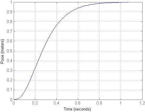
When applying the test effect in the form of a single step, we obtain the following result:

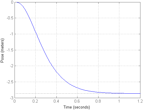
As you can see, it turns out that the object flew a fairly large distance with little impact, although it remained in the same position. In order for the input to correspond to the output, we can calculate the scaling factor km and multiply the input signal by it, which was implemented in the second model. Then the transition process will look like this:

The resulting position is still great for such an installation. For now, let us ignore the current and go directly to the Simulink models, where we will consider the remaining things.

We scale the input signal so that the output values ​​are conveniently represented in centimeters. We apply several test actions to the input to check how the transients in the system look, as well as the flowing current.

It turns out that the magnitude of the current at such positions of the object is not so significant. The transients themselves in position are aperiodic in nature, without overshoot and static error. Actually, it was set by the desired poles of the adjusted system.

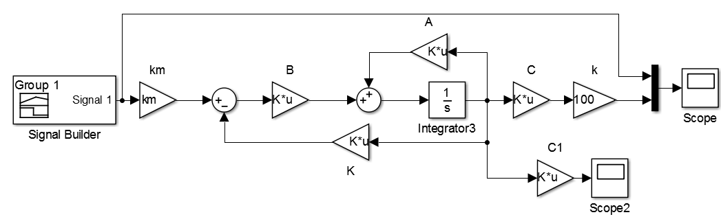
However, this approximation at the operating point may not work correctly with the original nonlinear model. Check this out. A non-linear system model with a connected controller is shown below.

This is the final version left after all the experiments. There were established restrictions on the input voltage (0-12V) and the position of the object itself (0-4cm). The second component of the regulator was excluded, since with it the transition process was unstable:

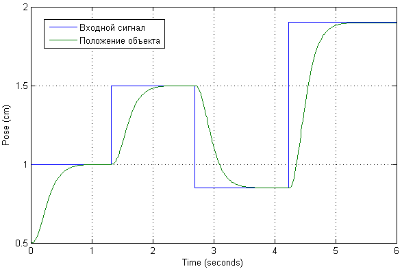
After changes to the circuit, transients now look like this:

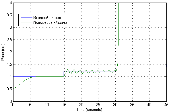
The possible range of operation of such a system was immediately checked. You can see that the desired position will be achieved with slight deviations from the starting point. In this case, a manifestation of significant oscillation is possible.

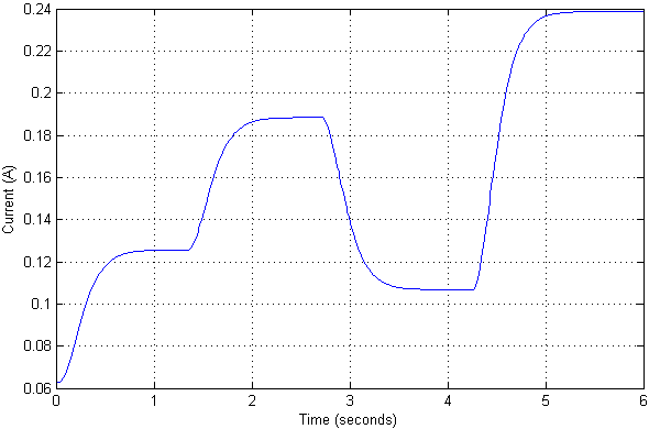
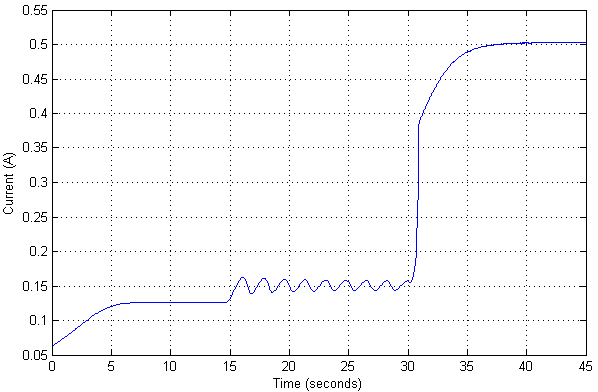
In this case, the current value is as follows:

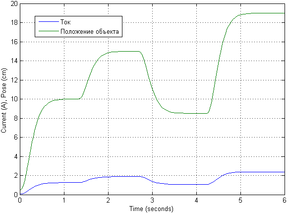
Once there has already been a check for a non-linear model of an object, then you can look at what the maximum position value for an object can be at which it still does not lose stability.

After modeling with different input signals, it was noticed that the linearized model is very good. So here we will demonstrate transients according to the initial input signal increased by 10 times.

The mathematical model itself might look a little different. Its description is taken from the description of the mathematical model .

Conclusion

Modal control for this nonlinear model of a magnetic levitation system is not at all suitable for any practical needs. Other implementations for this magnetic levitation system should be considered.

As for the bachelor's work, the author implemented a simple installation on levitation, which will be separately described in the future.