We design a space rocket from scratch. Part 2 - Semi-solution of the two-body problem

Content

Part 1 - The task of two bodies

Variable change trickery

Greetings to all! In the last part, we got the equations of motion of a system of two material points, as well as some motivation to use this model. Now let's try to squeeze as much information from them as possible. Here they are:

\ begin {equation *}

\ begin {cases}

m_ {1} \ ddot {\ vec {r}} _ {1} = \ vec {F} _ {12}, (1)

\\

m_ {2} \ ddot {\ vec {r}} _ {2} = - \ vec {F} _ {12},

\ end {cases}

\ end {equation *}

Where

v e c F_{12} = G d f r a c m_{1} m_{2} | v e c r_{2} - v e c r_{1} |^{3} l e f t (v e c r_{2} - v e c r_{1} r i g h t) .

$\ vec {F} _ {12} = G \ dfrac {m_ {1} m_ {2}} {| \ vec {r} _ {2} - \ vec {r} _ {1} | ^ {3} } \ left (\ vec {r} _ {2} - \ vec {r} _ {1} \ right).$

The system looks simple, especially if you close your eyes and do not look at the expression for

v e c F_{12}

$\ vec {F} _ {12}$ . Even, for a moment, it starts to seem that the equations are linear and solving it is a trivial matter. But the cube spoils the whole raspberry, and if you expand this whole thing and write it in phase coordinates, then our task is non-linear and generally in 12-dimensional space (not too lazy, typed):

\ begin {equation *}

\ begin {cases}

\ dot {x} _ {1} = v_ {1x}

\\

\ dot {y} _ {1} = v_ {1y}

\\

\ dot {z} _ {1} = v_ {1z}

\\

\ dot {v} _ {1x} = \ dfrac {G m_ {2} \ left (x_ {2} - x_ {1} \ right)} {\ left (\ sqrt {(x_ {2} - x_ {1 }) ^ {2} + (y_ {2} - y_ {1}) ^ {2} + (z_ {2} - z_ {1}) ^ {2}} \ right) ^ {3}}

\\

\ dot {v} _ {1y} = \ dfrac {G m_ {2} \ left (y_ {2} - y_ {1} \ right)} {\ left (\ sqrt {(x_ {2} - x_ {1 }) ^ {2} + (y_ {2} - y_ {1}) ^ {2} + (z_ {2} - z_ {1}) ^ {2}} \ right) ^ {3}}

\\

\ dot {v} _ {1z} = \ dfrac {G m_ {2} \ left (z_ {2} - z_ {1} \ right)} {\ left (\ sqrt {(x_ {2} - x_ {1 }) ^ {2} + (y_ {2} - y_ {1}) ^ {2} + (z_ {2} - z_ {1}) ^ {2}} \ right) ^ {3}}

\\

\ dot {x} _ {2} = v_ {2x}

\\

\ dot {y} _ {2} = v_ {2y}

\\

\ dot {z} _ {2} = v_ {2z}

\\

\ dot {v} _ {2x} = \ dfrac {G m_ {1} \ left (x_ {1} - x_ {2} \ right)} {\ left (\ sqrt {(x_ {2} - x_ {1 }) ^ {2} + (y_ {2} - y_ {1}) ^ {2} + (z_ {2} - z_ {1}) ^ {2}} \ right) ^ {3}}

\\

\ dot {v} _ {2y} = \ dfrac {G m_ {1} \ left (y_ {1} - y_ {2} \ right)} {\ left (\ sqrt {(x_ {2} - x_ {1 }) ^ {2} + (y_ {2} - y_ {1}) ^ {2} + (z_ {2} - z_ {1}) ^ {2}} \ right) ^ {3}}

\\

\ dot {v} _ {2z} = \ dfrac {G m_ {1} \ left (z_ {1} - z_ {2} \ right)} {\ left (\ sqrt {(x_ {2} - x_ {1 }) ^ {2} + (y_ {2} - y_ {1}) ^ {2} + (z_ {2} - z_ {1}) ^ {2}} \ right) ^ {3}}

\ end {cases}

\ end {equation *}

If we had written it like this at first, then we couldn’t see the forests behind these trees, but, thank God, He lifted us up to his Mount Zion and you can clearly see the whole forest from it (by the way, if you look at Siberia from space, we’ll see that the forest is burning) . And intuition will tell us what to do with equations 1. Em, add and there will be zero on the right:

m_{1} d d o t {v e c r}_{1} + m_{2} d d o t {v e c r}_{2} = 0

$m_ {1} \ ddot {\ vec {r}} _ {1} + m_ {2} \ ddot {\ vec {r}} _ {2} = 0$

Doesn’t resemble anything? And so:

f r a c m_{1} d d o t {v e c r}_{1} + m_{2} d d o t {v e c r}_{2} m_{1} + m_{2} = 0, (2)

$\ frac {m_ {1} \ ddot {\ vec {r}} _ {1} + m_ {2} \ ddot {\ vec {r}} _ {2}} {m_ {1} + m_ {2} } = 0, (2)$

Center of mass of the system:

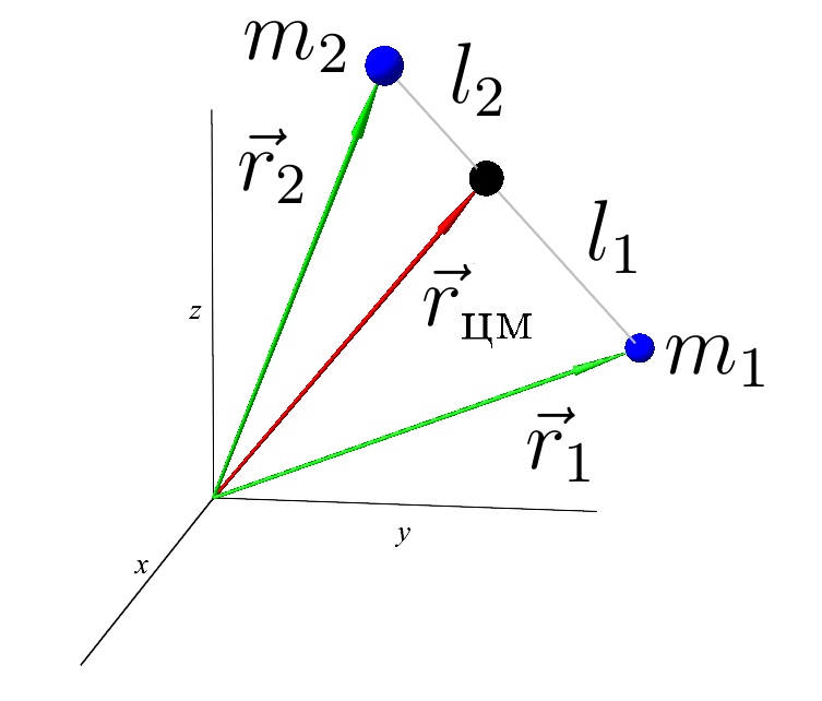
v e c r_{t e x t c m} = f r a c m_{1} v e c r_{1} + m_{2} v e c r_{2} m_{1} + m_{2},

$\ vec {r} _ {\ text {cm}} = \ frac {m_ {1} \ vec {r} _ {1} + m_ {2} \ vec {r} _ {2}} {m_ {1 } + m_ {2}},$

The center of mass of two bodies. Distance relationship

$l_ {1}$ and

$l_ {2}$ equal to the ratio of the masses. But in this order, so that the center of mass is closer to a heavier body.

which means from 2 it follows that the acceleration of the center of mass of the system is zero:

d d o t {v e c r}_{t e x t c m} = 0, (3)

$\ ddot {\ vec {r}} _ {\ text {cm}} = 0, (3)$

but this is the same as Newton’s first law. It turns out that the center of mass will always and everywhere move rectilinearly at a constant speed, or remain in place. We integrate 3 a couple of times (here it’s like a system of diffurs, but each coordinate is integrated independently of the others):

d o t {v e c r}_{t e x t c m} = v e c C_{1},

$\ dot {\ vec {r}} _ {\ text {cm}} = \ vec {C} _ {1},$

v e c r_{t e x t c m} = v e c C_{1} t + v e c C_{2},

$\ vec {r} _ {\ text {cm}} = \ vec {C} _ {1} t + \ vec {C} _ {2},$

Where

v e c C_{1}, v e c C_{2}

$\ vec {C} _ {1}, \ vec {C} _ {2}$ - vector constants, which are (dimensional analysis) the initial velocity and the initial position of the center of mass, respectively. Well, and rewrite:

v e c r_{t e x t c m} = v e c v_{t e x t c m} t + v e c r_{t e x t c m},

$\ vec {r} _ {\ text {cm}} = \ vec {v} _ {\ text {cm}} t + \ vec {r} _ {\ text {cm}},$

It is easy to recalculate the initial conditions:

v e c r_{t e x t c m 0} = f r a c m_{1} v e c r_{10} + m_{2} v e c r_{20} m_{1} + m_{2},

$\ vec {r} _ {\ text {cm0}} = \ frac {m_ {1} \ vec {r} _ {10} + m_ {2} \ vec {r} _ {20}} {m_ {1 } + m_ {2}},$

v e c v_{t e x t c m 0} = f r a c m_{1} v e c v_{10} + m_{2} v e c v_{20} m_{1} + m_{2},

$\ vec {v} _ {\ text {cm0}} = \ frac {m_ {1} \ vec {v} _ {10} + m_ {2} \ vec {v} _ {20}} {m_ {1 } + m_ {2}},$

but

v e c r_{10} = v e c r_{1} (0), v e c r_{20} = v e c r_{2} (0), v e c v_{10} = d o t {v e c r}_{1} (0), v e c v_{20} = d o t {v e c r}_{2} (0)

$\ vec {r} _ {10} = \ vec {r} _ {1} (0), \ vec {r} _ {20} = \ vec {r} _ {2} (0), \ vec { v} _ {10} = \ dot {\ vec {r}} _ {1} (0), \ vec {v} _ {20} = \ dot {\ vec {r}} _ {2} (0)$ - so that there is no understatement. I forgot at the beginning to say that all these initial conditions together with equations 1 form the Cauchy problem, which, as is known from the section of matan with diffurs, has clearly one solution for each initial condition. And this is good, because there are more complicated tasks, for example, boundary ones. When part of the phase coordinates is specified at one point, part at another point. It happens that the position is known at the beginning, and the speed should be such at the end. But there is no initial speed. And I feel that we will have to solve such problems in the future too;)

You can even check how the center of mass moves by solving the problem numerically. An old laptop on which I work, will allow to model it:

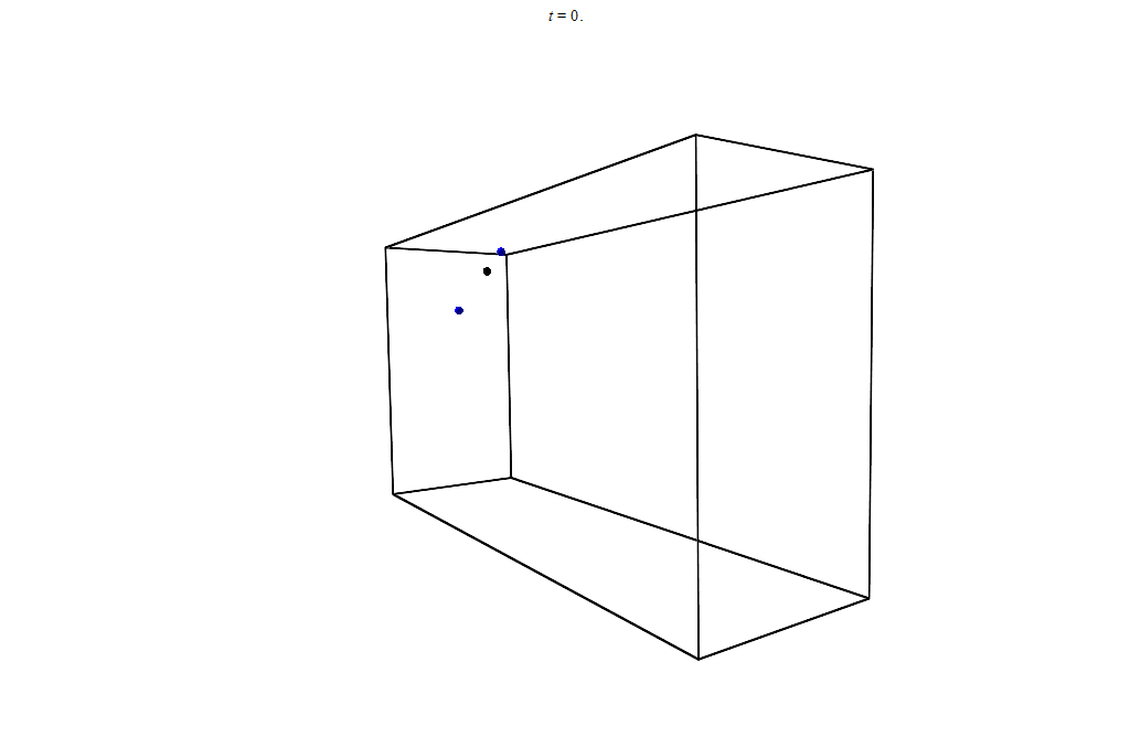
Animation of the movement of bodies and the center of mass. Numerical solution

Oh well. We figured out how the center of mass moves, but this is not enough! I want to know how the bodies move. Take another look at the system:

\ begin {equation *}

\ begin {cases}

m_ {1} \ ddot {\ vec {r}} _ {1} = G \ dfrac {m_ {1} m_ {2}} {| \ vec {r} _ {2} - \ vec {r} _ { 1} | ^ {3}} \ left (\ vec {r} _ {2} - \ vec {r} _ {1} \ right),

\\

m_ {2} \ ddot {\ vec {r}} _ {2} = -G \ dfrac {m_ {1} m_ {2}} {| \ vec {r} _ {2} - \ vec {r} _ {1} | ^ {3}} \ left (\ vec {r} _ {2} - \ vec {r} _ {1} \ right),

\ end {cases}

\ end {equation *}

or

\ begin {equation *}

\ begin {cases}

\ ddot {\ vec {r}} _ {1} = G \ dfrac {m_ {2}} {| \ vec {r} _ {2} - \ vec {r} _ {1} | ^ {3}} \ left (\ vec {r} _ {2} - \ vec {r} _ {1} \ right),

\\

\ ddot {\ vec {r}} _ {2} = -G \ dfrac {m_ {1}} {| \ vec {r} _ {2} - \ vec {r} _ {1} | ^ {3} } \ left (\ vec {r} _ {2} - \ vec {r} _ {1} \ right),

\ end {cases}

\ end {equation *}

And there, and there is a difference on the right

v e c r_{2} - v e c r_{1},

$\ vec {r} _ {2} - \ vec {r} _ {1},$ so let's do it quick:

d d o t {v e c r}_{2} - d d o t {v e c r}_{1} = - G d f r a c m_{1} | v e c r_{2} - v e c r_{1} |^{3} l e f t (v e c r_{2} - v e c r_{1} r i g h t) - G d f r a c m_{2} | v e c r_{2} - v e c r_{1} |^{3} l e f t (v e c r_{2} - v e c r_{1} r i g h t),

$\ ddot {\ vec {r}} _ {2} - \ ddot {\ vec {r}} _ {1} = -G \ dfrac {m_ {1}} {| \ vec {r} _ {2} - \ vec {r} _ {1} | ^ {3}} \ left (\ vec {r} _ {2} - \ vec {r} _ {1} \ right) - G \ dfrac {m_ {2} } {| \ vec {r} _ {2} - \ vec {r} _ {1} | ^ {3}} \ left (\ vec {r} _ {2} - \ vec {r} _ {1} \ right),$

d f r a c d^{2} d t^{2} l e f t (v e c r_{2} - v e c r_{1} r i g h t) = - G d f r a c (m_{1} + m_{2}) | v e c r_{2} - v e c r_{1} |^{3} l e f t (v e c r_{2} - v e c r_{1} r i g h t),

$\ dfrac {d ^ {2}} {dt ^ {2}} \ left (\ vec {r} _ {2} - \ vec {r} _ {1} \ right) = -G \ dfrac {(m_ {1} + m_ {2})} {| \ vec {r} _ {2} - \ vec {r} _ {1} | ^ {3}} \ left (\ vec {r} _ {2} - \ vec {r} _ {1} \ right),$

previously we designated the difference as

v e c r_{12} = v e c r_{2} - v e c r_{1},

$\ vec {r} _ {12} = \ vec {r} _ {2} - \ vec {r} _ {1},$ but now reassign

v e c r = v e c r_{2} - v e c r_{1},

$\ vec {r} = \ vec {r} _ {2} - \ vec {r} _ {1},$ since it’s necessary (I’ll say in advance) to work with this thing more than once. Well, remember, and then the last equality will take the form:

d d o t v e c r = - G d f r a c (m_{1} + m_{2}) r^{3} v e c r,

$\ ddot {\ vec {r}} = -G \ dfrac {(m_ {1} + m_ {2})} {r ^ {3}} \ vec {r},$

either like this:

d d o t v e c r = - m u d f r a c v e c r r^{3}, (4)

$\ ddot {\ vec {r}} = - \ mu \ dfrac {\ vec {r}} {r ^ {3}}, (4)$

Where

m u = G (m_{1} + m_{2}) > 0,

$\ mu = G (m_ {1} + m_ {2})> 0,$ but

v e c r

$\ vec {r}$ - the relative distance between the bodies. Start of vector

v e c r

$\ vec {r}$ at material point number 1, and the end at point 2.

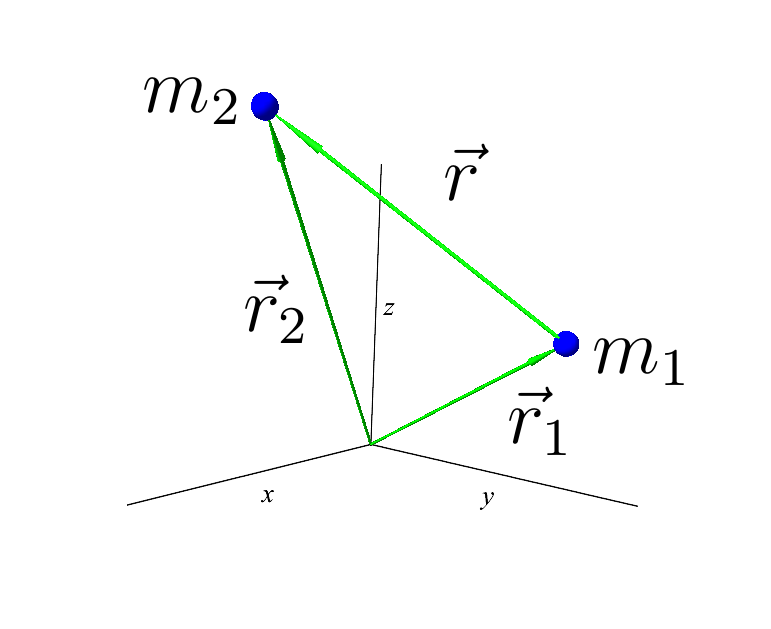
Vector

$\ vec {r}$

In fact, all these tricks with the center of mass and relative distance are a linear transformation of variables:

\ begin {equation *}

\ begin {cases}

\ vec {r} _ {1} = \ alpha_ {1} \ vec {r} _ {\ text {cm}} + \ beta_ {1} \ vec {r},

\\

\ vec {r} _ {2} = \ alpha_ {2} \ vec {r} _ {\ text {cm}} + \ beta_ {2} \ vec {r},

\ end {cases}

\ end {equation *}

but so far it’s written the other way around:

\ begin {equation *}

\ begin {cases}

\ vec {r} _ {\ text {cm}} = \ frac {m_ {1} \ vec {r} _ {1} + m_ {2} \ vec {r} _ {2}} {m_ {1} + m_ {2}},

\\

\ vec {r} = \ vec {r} _ {2} - \ vec {r} _ {1},

\ end {cases}

\ end {equation *}

or

\ begin {equation *}

\ begin {cases}

\ vec {r} _ {\ text {cm}} = \ dfrac {m_ {1}} {(m_ {1} + m_ {2})} \ vec {r} _ {1} + \ dfrac {m_ { 2}} {(m_ {1} + m_ {2})} \ vec {r} _ {2},

\\

\ vec {r} = - \ vec {r} _ {1} + \ vec {r} _ {2},

\ end {cases}

\ end {equation *}

could be so:

\ begin {bmatrix} \ dfrac {m_ {1}} {(m_ {1} + m_ {2})} & \ dfrac {m_ {2}} {(m_ {1} + m_ {2})} \ \ -1 & 1 \ end {bmatrix} \ begin {bmatrix} \ vec {r} _ {1} \\ \ vec {r} _ {2} \ end {bmatrix} = \ begin {bmatrix} \ vec {r } _ {\ text {cm}} \\ \ vec {r} \ end {bmatrix}

$\ begin {bmatrix} \ dfrac {m_ {1}} {(m_ {1} + m_ {2})} & \ dfrac {m_ {2}} {(m_ {1} + m_ {2})} \ \ -1 & 1 \ end {bmatrix} \ begin {bmatrix} \ vec {r} _ {1} \\ \ vec {r} _ {2} \ end {bmatrix} = \ begin {bmatrix} \ vec {r } _ {\ text {cm}} \\ \ vec {r} \ end {bmatrix}$

And now multiplying by the inverse matrix on the left (or in what other way to solve this system), we can express:

\ begin {equation *}

\ begin {cases}

\ vec {r} _ {1} = \ vec {r} _ {\ text {cm}} - \ dfrac {m_ {2}} {m_ {1} + m_ {2}} \ vec {r}, ( five)

\\

\ vec {r} _ {2} = \ vec {r} _ {\ text {cm}} + \ dfrac {m_ {1}} {m_ {1} + m_ {2}} \ vec {r}.

\ end {cases}

\ end {equation *}

This transformation allowed us to divide the problem into two independent ones: separately find the motion of the center of mass and separately the relative distance. And through them already express the movement in the global coordinate system. So we have already decided the floor of the problem - we know how the center of mass moves. Now having solved 4 the problem will be considered completely solved. But this is the next time.

Now, we should add the analysis of equations 5. In the case when one of the bodies will be much more massive than the other (approx. Earth and Man, or Earth and apple of Man). Let's take the first body massive, the second one not so:

m_{1} >> m_{2}

$m_ {1} >> m_ {2}$ or

d f r a c m_{2} m_{1} << 1,

$\ dfrac {m_ {2}} {m_ {1}} << 1,$ What means

d f r a c m_{2} m_{1} = 0.000001 a p p r o x 0.

$\ dfrac {m_ {2}} {m_ {1}} = 0.000001 \ approx 0.$

In this case:

v e c r_{t e x t c m} = f r a c m_{1} v e c r_{1} + m_{2} v e c r_{2} m_{1} + m_{2} = d f r a c m_{1} m_{1} f r a c v e c r_{1} + d f r a c m_{2} m_{1} v e c r_{2} 1 + d f r a c m_{2} m_{1} a p p r o x f r a c v e c r_{1} + 0 v e c r_{2} 1 + 0 = v e c r_{1},

$\ vec {r} _ {\ text {cm}} = \ frac {m_ {1} \ vec {r} _ {1} + m_ {2} \ vec {r} _ {2}} {m_ {1 } + m_ {2}} = \ dfrac {m_ {1}} {m_ {1}} \ frac {\ vec {r} _ {1} + \ dfrac {m_ {2}} {m_ {1}} \ vec {r} _ {2}} {1 + \ dfrac {m_ {2}} {m_ {1}}} \ approx \ frac {\ vec {r} _ {1} + 0 \ vec {r} _ { 2}} {1 + 0} = \ vec {r} _ {1},$

- which means the concentration of the center of mass of the system directly in a massive body

m_{1},

$m_ {1},$

\ begin {equation *}

\ begin {cases}

\ vec {r} _ {1} = \ vec {r} _ {\ text {cm}} - \ dfrac {1} {m_ {1}} \ dfrac {m_ {2}} {1 + \ dfrac {m_ {2}} {m_ {1}}} \ vec {r} = \ vec {r} _ {\ text {cm}} - \ dfrac {m_ {2}} {m_ {1}} \ dfrac {1} {1 + 0} \ vec {r},

\\

\ vec {r} _ {2} = \ vec {r} _ {\ text {cm}} + \ dfrac {1} {m_ {1}} \ dfrac {m_ {1}} {1 + \ dfrac {m_ {2}} {m_ {1}}} \ vec {r} = \ vec {r} _ {\ text {cm}} + \ dfrac {m_ {1}} {m_ {1}} \ dfrac {1} {1 + 0} \ vec {r}.

\ end {cases}

\ end {equation *}

Finally:

\ begin {equation *}

\ begin {cases}

\ vec {r} _ {1} = \ vec {r} _ {\ text {cm}},

\\

\ vec {r} _ {2} = \ vec {r} _ {\ text {cm}} + \ vec {r}.

\ end {cases}

\ end {equation *}

Now, if we transfer the original coordinate system to the center of mass, we get:

\ begin {equation *}

\ begin {cases}

\ vec {r} _ {1} = 0,

\\

\ vec {r} _ {2} = \ vec {r}.

\ end {cases}

\ end {equation *}

That is, we have connected the new coordinate system with the Earth. And the Earth in its own coordinate. the system is motionless. Vector

v e c r

$\ vec {r}$ here already is just the radius of the vector, but at the same time remains the relative distance between the bodies.

So in the next article, solving this equation:

d d o t v e c r = - m u d f r a c v e c r r^{3},

$\ ddot {\ vec {r}} = - \ mu \ dfrac {\ vec {r}} {r ^ {3}},$

can be interpreted

v e c r

$\ vec {r}$ as the position of a satellite in a coordinate system associated with the Earth, for example.

Although deciding it, this is completely optional. The solution will be for two arbitrary bodies (arbitrary masses).

To be continued…

Literature:

Balk M.B. Elements of the dynamics of space flight, Moscow: Nauka, Glav.red.phys.-math. Lit., 1965. - 338s.

All Articles

We design a space rocket from scratch. Part 2 - Semi-solution of the two-body problem

Content

Variable change trickery

More articles: