トレーダーの伝説の1つは、「機関車」の概念です。 次のように説明できます。「主要な」論文と「導かれた」論文があります。 このようなパターンの存在を信じている場合、「機関車」(「主要な」証券)の動きによって、金融商品の将来の動きを「予測」できます。 そうですか? これには理由がありますか?

問題を定式化します。 金融商品があります:A、B、C、D。 時間の特性があります-t。 これらの楽器の動きの間には何らかのつながりがありますか?
A tおよびB t-1 ; A tおよびC t-1 ; A tおよびD t-1
B tおよびC t-1 ; B tおよびD t-1 ; B tおよびA t-1
C tおよびD t-1 ; C tおよびA t-1 ; C tおよびB t-1
D tおよびA t-1 ; D tおよびB t-1 ; D tおよびB t-1
この問題を研究するためのデータを取得する方法は? リンクはどれほど強力で安定していますか? それらはどのように測定できますか? どんなツール?
 まず、今日ではかなりの数の予測モデルがあることに注意してください。 いくつかの情報源は、それらの数が100を超えたと言います。 ちなみに、現実の主な冗談は... ...モデルが複雑になるほど、解釈が難しくなり、このモデル自体の個々のコンポーネントを理解することです。 この記事の目的は、上記の質問に答えることであり、既存の予測モデルを使用することではないことを強調します。
pandasパッケージは、豊富なツールを備えた強力なデータ分析ツールです。 私たちはその機能を使用して質問を研究します。
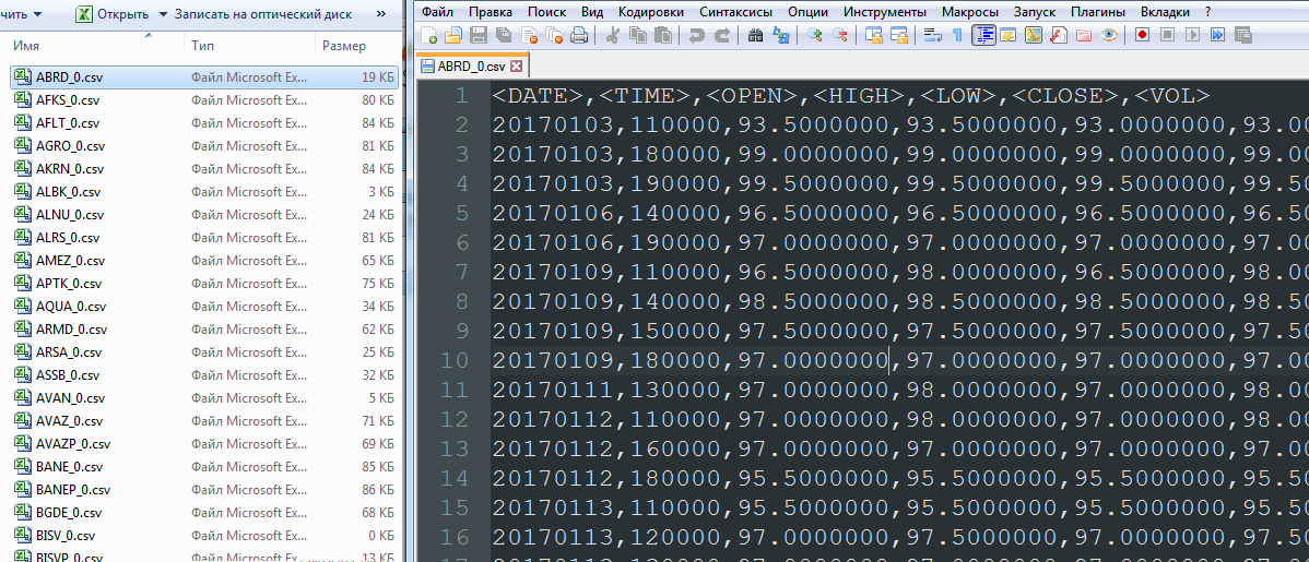
事前に、FINAM会社のサーバーから見積もりを受け取ります。 2017年1月1日から2017年7月13日までの期間の「監視」を行います。 ここで言及した関数をわずかに変更することにより、次のようになります。
# -*- coding: utf-8 -*- """ @author: optimusqp """ import os import urllib import pandas as pd import time import codecs from datetime import datetime, date from pandas.io.common import EmptyDataError e='.csv'; p='7'; yf='2017'; yt='2017'; month_start='01'; day_start='01'; month_end='07'; day_end='13'; year_start=yf[2:]; year_end=yt[2:]; mf=(int(month_start.replace('0','')))-1; mt=(int(month_end.replace('0','')))-1; df=(int(day_start.replace('0',''))); dt=(int(day_end.replace('0',''))); dtf='1'; tmf='1'; MSOR='1'; mstimever='0' sep='1'; sep2='1'; datf='5'; at='1'; def quotes_finam_optimusqp(data,year_start,month_start,day_start,year_end,month_end,day_end,e,df,mf,yf,dt,mt,yt,p,dtf,tmf,MSOR,mstimever,sep,sep2,datf,at): temp_name_file='id,company\n'; incrim=1; for index, row in data.iterrows(): page = urllib.urlopen('http://export.finam.ru/'+str(row['code'])+'_'+str(year_start)+str(month_start)+str(day_start)+'_'+str(year_end)+str(month_end)+str(day_end)+str(e)+'?market='+str(row['id_exchange_2'])+'&em='+str(row['em'])+'&code='+str(row['code'])+'&apply=0&df='+str(df)+'&mf='+str(mf)+'&yf='+str(yf)+'&from='+str(day_start)+'.'+str(month_start)+'.'+str(yf)+'&dt='+str(dt)+'&mt='+str(mt)+'&yt='+str(yt)+'&to='+str(day_end)+'.'+str(month_end)+'.'+str(yt)+'&p='+str(p)+'&f='+str(row['code'])+'_'+str(year_start)+str(month_start)+str(day_start)+'_'+str(year_end)+str(month_end)+str(day_end)+'&e='+str(e)+'&cn='+str(row['code'])+'&dtf='+str(dtf)+'&tmf='+str(tmf)+'&MSOR='+str(MSOR)+'&mstimever='+str(mstimever)+'&sep='+str(sep)+'&sep2='+str(sep2)+'&datf='+str(datf)+'&at='+str(at)) print('http://export.finam.ru/'+str(row['code'])+'_'+str(year_start)+str(month_start)+str(day_start)+'_'+str(year_end)+str(month_end)+str(day_end)+str(e)+'?market='+str(row['id_exchange_2'])+'&em='+str(row['em'])+'&code='+str(row['code'])+'&apply=0&df='+str(df)+'&mf='+str(mf)+'&yf='+str(yf)+'&from='+str(day_start)+'.'+str(month_start)+'.'+str(yf)+'&dt='+str(dt)+'&mt='+str(mt)+'&yt='+str(yt)+'&to='+str(day_end)+'.'+str(month_end)+'.'+str(yt)+'&p='+str(p)+'&f='+str(row['code'])+'_'+str(year_start)+str(month_start)+str(day_start)+'_'+str(year_end)+str(month_end)+str(day_end)+'&e='+str(e)+'&cn='+str(row['code'])+'&dtf='+str(dtf)+'&tmf='+str(tmf)+'&MSOR='+str(MSOR)+'&mstimever='+str(mstimever)+'&sep='+str(sep)+'&sep2='+str(sep2)+'&datf='+str(datf)+'&at='+str(at)) print('code: '+str(row['code'])) # . # - file = codecs.open(str(row['code'])+"_"+"0"+".csv", "w", "utf-8") content = page.read() file.write(content) file.close() temp_name_file = temp_name_file + (str(incrim) + "," + str(row['code'])+"\n") incrim+=1 time.sleep(2) # code , # - . write_file = "name_file_data.csv" with open(write_file, "w") as output: for line in temp_name_file: output.write(line) # quotes_finam_optimusqp # function_parameters.csv #___http://optimusqp.ru/articles/articles_1/function_parameters.csv data_all = pd.read_csv('function_parameters.csv', index_col='id') # , # id_exchange_2 == 1, .. data = data_all[data_all['id_exchange_2']==1] quotes_finam_optimusqp(data,year_start,month_start,day_start,year_end,month_end,day_end,e,df,mf,yf,dt,mt,yt,p,dtf,tmf,MSOR,mstimever,sep,sep2,datf,at)
その結果、タイプA_0.csvのファイルのリストがあります。
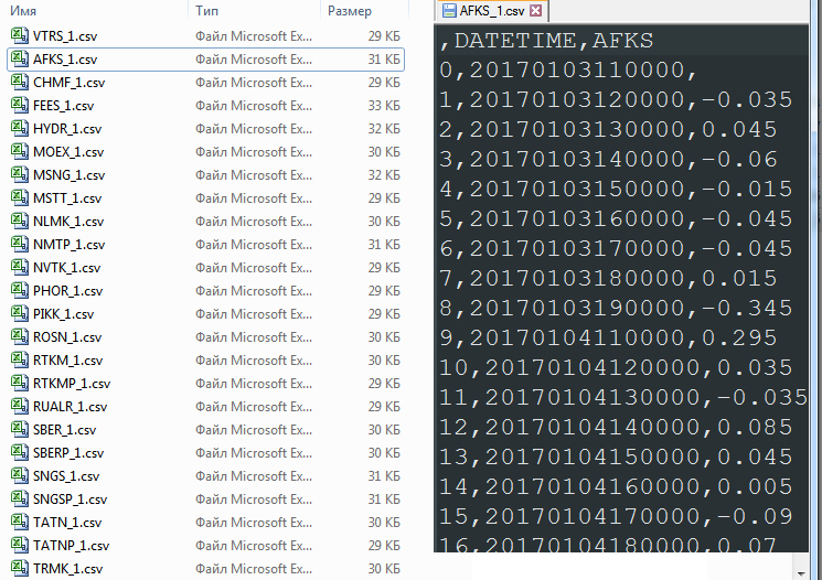
次に、金融商品A t -A t-1の動きを決定し、OPEN、HIGH、LOW、VOLの列を削除して、DATETIMEという単一の列を形成します。 分析するデータが少なすぎる(最近取引された、不安定、または流動性がほとんどない)金融商品を選別します。
# , ? # - . name_file_data = pd.read_csv('name_file_data.csv', index_col='id') incrim=1; # how_work_days - , # , # temp_string_in_file='id,how_work_days\n'; for index, row1 in name_file_data.iterrows(): how_string_in_file = 0 # , name_file=row1['company']+"_"+"0"+".csv" # ? if os.path.exists(name_file): folder_size = os.path.getsize(name_file) # - , if folder_size>0: temp_quotes_data=pd.read_csv(name_file, delimiter=',') # , EmptyDataError # try: # (CLOSE); # quotes_data = temp_quotes_data.drop(['<OPEN>', '<HIGH>', '<LOW>', '<VOL>'], axis=1) # - how_string_in_file = len(quotes_data.index) # 1 100, # ; if how_string_in_file>1100: # days_data.csv, # # temp_string_in_file = temp_string_in_file + (str(incrim) + "," + str(how_string_in_file)+"\n") incrim+=1 quotes_data['DATE_str']=quotes_data['<DATE>'].astype(basestring) quotes_data['TIME_str']=quotes_data['<TIME>'].astype(basestring) #"" DATETIME quotes_data['DATETIME'] = quotes_data.apply(lambda x:'%s%s' % (x['DATE_str'],x['TIME_str']),axis=1) quotes_data = quotes_data.drop(['<DATE>','<TIME>','DATE_str','TIME_str'], axis=1) quotes_data['DATETIME'].apply(lambda d: datetime.strptime(d, '%Y%m%d%H%M%S')) quotes_data [row1['company']] = quotes_data['<CLOSE>'] - quotes_data['<CLOSE>'].shift(1) quotes_data = quotes_data.drop(['<CLOSE>'], axis=1) quotes_data.to_csv(row1['company']+"_"+"1"+".csv", sep=',', encoding='utf-8') os.unlink(row1['company']+"_"+"0"+".csv") else: os.unlink(row1['company']+"_"+"0"+".csv") except pd.io.common.EmptyDataError: os.unlink(row1['company']+"_"+"0"+".csv") else: os.unlink(row1['company']+"_"+"0"+".csv") else: continue write_file = "days_data.csv" with open(write_file, "w") as output: for line in temp_string_in_file: output.write(line)
その結果、タイプA_1.csvのファイルのリストを取得します。 合計91ファイル:
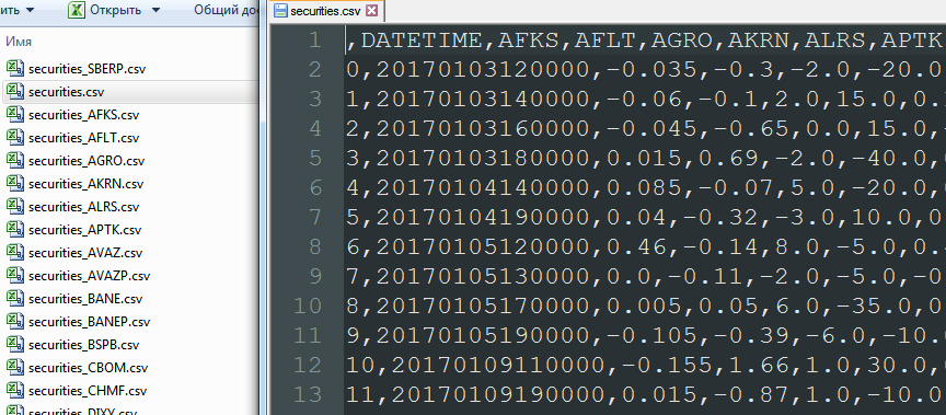
すべての金融商品のすべての動きを1つの有価証券.csvファイルにマージし、最初の空行を削除します。
import glob allFiles = glob.glob("*_1.csv") frame = pd.DataFrame() list_ = [] for file_ in allFiles: df = pd.read_csv(file_,index_col=None, header=0) list_.append(df) dfff = reduce(lambda df1,df2: pd.merge(df1,df2,on='DATETIME'), list_) quotes_data = dfff.drop(['Unnamed: 0_x', 'Unnamed: 0_y', 'Unnamed: 0'], axis=1) quotes_data.to_csv("securities.csv", sep=',', encoding='utf-8') quotes_data = quotes_data.drop(['DATETIME'], axis=1) number_columns=len(quotes_data.columns) columns_name_0 = quotes_data.columns columns_name_1 = quotes_data.columns
この段階で、DATETIME列(pd.merge)によってレコードを結合するかなり興味深い操作が行われます。 この統合命令は、91の証券のうち少なくとも1つが取引されなかった日付を破棄します。 つまり、結合は空のデータの完全な除外に基づいています。 その結果:
ループ内のデータを操作するSecurities.csvファイルでは、現在の行を除くすべての行をシフトします。 したがって、A tの反対側には、B t-1 、C t-1 、D t-1の値があります。
incrim=0 quotes_data_w=quotes_data.shift(1) for column in columns_name_0: quotes_data_w[column]=quotes_data_w[column].shift(-1) quotes_data_w.to_csv("securities_"+column+".csv", sep=',', encoding='utf-8') # quotes_data_w[column]=quotes_data_w[column].shift(1) incrim+=1
データは次のようになります。

そして、はい、空のデータを持つ最初の行を削除する必要があります。 これで、列間の相関を構築できます。 彼らは、「機関車」論文の有無を明らかにするか、「機関車」が神話に過ぎないことを確認できるようにします。
金融商品の動きに正規(ガウス)分布がないという事実は、比較的最近議論されてきました。 ただし、ほとんどの財務モデルは、その仮定に基づいて正確に構築されます。 データにガウス分布がありますか? 正規性の存在はピアソン相関の使用を可能にし、不在はノンパラメトリックタイプの相関の使用を余儀なくされるので、質問は怠idleではありません。 この質問で、私たちは素晴らしい陰謀的なサービスに目を向けます。
 このサービスの何が面白いですか? まず、グラフィカルにデータを解釈する機能。 第二に、統計的検定方法のセット。 特に、サンプルが正規(ガウス)分布に準拠しているかどうかをテストする能力。 次のテストを使用します。Shapiro-Wilk基準(Shapiro-Wilk)、Kolmogorov-Smirnov基準(Kolmogorov-Smirnov)は、 ここで作業規則を参照してください 。
陰謀的なサービスは最高の賞賛に値します。 Linuxでのplotlyの構成に関するチュートリアルは、 plot.lyで見ることができますが、Windowsの場合は、たとえばこちらをご覧ください 。 しかしplotlyにはいくつかの奇妙な点があります。 そして、ここでの質問は、テストのロジックの説明に劣らない。 使用例では、テーブルが与えられます:

開発者は次のコメントを提供します。
p値はテスト統計よりもはるかに小さいため、0.05の有意水準で帰無仮説を棄却しない良い証拠があります。
翻訳:
p値は検定統計量よりもはるかに小さいため、有意水準0.05で帰無仮説を放棄していないという十分な証拠があります。
したがって、この勧告によれば、 検討中のサンプルの分布の正規性に関する仮説を放棄する権利はありません! しかし...このアドバイスは真実ではありません 。
覚えておいてください-p値とは何ですか? この値は、統計的仮説をテストするために必要です。 帰無仮説を棄却した場合、エラーの確率として理解できます。 Shapiro-Wilk基準H 0の帰無仮説では、「ランダム変数Xは正規分布している」ということを思い出します。 極端に小さいp値(ゼロに近い)でH 0を拒否する場合、間違えられません。 分布が正常であるという仮定を除き、誤解することはありません。 一般に、正規性のプロット検定の有意水準は0.05であり、帰無仮説の受け入れまたは非受け入れは、この値とp-valueの比較に基づいている必要があります 。 有意水準のしきい値をp値で超えることは、テストサンプルの分布が正常であるという仮説を拒否できないことを意味します。

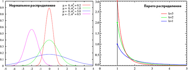
そして...突然、そして... plotlyの分布の正規性のテストは正しくありませんか? 先を見て、私は言います-すべてが順調です。 ガウスとパレートの2種類のランダムサンプルを生成しました。 これらのデータ配列は順次plot.lyに送信されます。 テスト中です。 分布の性質は非常に異なり、パレートサンプルが「正規性」のテストに合格しないことは明らかです。
テストコード:
import pandas as pd import matplotlib.pyplot as plt import plotly.plotly as py import plotly.graph_objs as go from plotly.tools import FigureFactory as FF import numpy as np from scipy import stats, optimize, interpolate def Normality_Test(L): x = L shapiro_results = scipy.stats.shapiro(x) matrix_sw = [ ['', 'DF', 'Test Statistic', 'p-value'], ['Sample Data', len(x) - 1, shapiro_results[0], shapiro_results[1]] ] shapiro_table = FF.create_table(matrix_sw, index=True) py.iplot(shapiro_table, filename='pareto_file') #py.iplot(shapiro_table, filename='normal_file') #L =np.random.normal(115.0, 10, 860) L =np.random.pareto(3,50) Normality_Test(L)
plot.ly/organize/homeのプロファイルで処理結果を確認できます
したがって、Shapiro-Wilkのテスト結果の一部を次に示します。
パレート分布の場合
最初のテスト

二次試験

正規(ガウス)分布の場合
最初のテスト

二次試験

したがって、テストアルゴリズムは正しく機能します。 ただし、テストを使用するためのヒントは、控えめに言っても、真実ではありません。 教訓は次のとおりです。 正しく書かれた楽器の近くに、正しく書かれた指示が常にあるとは限りません!
plotlyライブラリを使用して、正規性(ガウス)分布の金融商品の動きのテストに移りましょう。 次の結果が得られました。
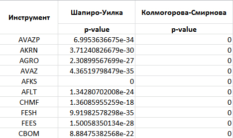
他の金融商品についても同様の状況。 したがって、問題の金融商品の動きの分布は正常であるという仮定を除外します。 テスト自体のコード:
allFiles = glob.glob("*_1.csv") def Shapiro(df,temp_header): df=df.drop(df.index[0]) x = df[temp_header].tolist() shapiro_results = scipy.stats.shapiro(x) matrix_sw = [ ['', 'DF', 'Test Statistic', 'p-value'], ['Sample Data', len(x) - 1, shapiro_results[0], shapiro_results[1]] ] shapiro_table = FF.create_table(matrix_sw, index=True) py.iplot(shapiro_table, filename='shapiro-table_'+temp_header) def Kolmogorov_Smirnov(df,temp_header): df=df.drop(df.index[0]) x = df[temp_header].tolist() ks_results = scipy.stats.kstest(x, cdf='norm') matrix_ks = [ ['', 'DF', 'Test Statistic', 'p-value'], ['Sample Data', len(x) - 1, ks_results[0], ks_results[1]] ] ks_table = FF.create_table(matrix_ks, index=True) py.iplot(ks_table, filename='ks-table_'+temp_header) frame = pd.DataFrame() list_ = [] for file_ in allFiles: df = pd.read_csv(file_,index_col=None, header=0) print(file_) columns = df.columns temp_header = columns[2] Shapiro(df,temp_header) time.sleep(3) Kolmogorov_Smirnov(df,temp_header) time.sleep(3)
分布の正規性(ガウス)に依存することはできないため、相関を計算するときは、ノンパラメトリックツール、つまりスピアマンランク相関係数を選択する必要があります 。 相関のタイプを決定したら、その計算に直接進むことができます。
incrim=0 for column0 in columns_name_1: df000 = pd.read_csv('securities_'+column0+".csv",index_col=None, header=0) # df000=df000.drop(df000.index[0]) df000 = df000.drop(['Unnamed: 0'], axis=1) # # corr_spr=df000.corr('spearman') # # corr_spr=corr_spr.sort_values([column0], ascending=False) # DataFrame corr_spr_temp=corr_spr[column0] corr_spr_temp.to_csv("corr_"+column0+".csv", sep=',', encoding='utf-8') incrim+=1
現在の論文(corr_A.csvなど)と他の証券の前期間(B、C、Dは90のみ)の相関関係を持つファイルを取得します。このため、securitys_A.csvタイプのファイルの空の値を持つ最初の行を削除します。 現在の証券に対する他の証券の相関を計算します。 相関の列をソートし、それらに名前を付けます。 現在のセキュリティの相関列を別のDataFrameとして保存します。

次に、corr_A.csvタイプの相関を持つ各ファイルを1つの共通ファイル_quotes_data_end.csv .csvにマージします。 このファイルの行は非パーソナライズされています。 ソートされた相関の値のみが観察できます。
incrim=0 all_corr_Files = glob.glob("corr_*.csv") list_corr = [] quotes_data_end = pd.DataFrame() for file_corr in all_corr_Files: df_corr = pd.read_csv(file_corr,index_col=None, header=0) columns_corr = df_corr.columns temp_header = columns_corr[0] quotes_data_end[str(temp_header)]=df_corr.iloc[:,1] incrim+=1 quotes_data_end.to_csv("_quotes_data_end.csv", sep=',', encoding='utf-8') plt.figure(); quotes_data_end.plot();

受信したデータ_quotes_data_end.csvに基づいて、グラフを作成します。

極端な地域でも相関のレベルは高くありません。 相関値の大部分は-0.15、0.15の範囲です。 そのため、検討期間(7.5か月)およびこの期間(「監視」)内に他の金融商品を「実行」する証券はありません。 91の証券に関するデータがあることを思い出させてください。 しかし...短い期間で同じ「ウォッチ」を処理しようとすると? 1か月のサンプルでは、次のグラフが得られます。

時間枠を短くし、検討中のサンプルのサイズを小さくすると、より高い相関が得られます。 「機関車」運動の神話(ある紙がそれと一緒に別の紙を「引っ張る」、または「カウンターバランス」として機能するとき)... が現実になります。 この効果は、サンプルサイズが減少するにつれて観察されます 。 ただし、コインの裏側はこの場合相関値の増加であるため、ますます不安定な動作を伴います 。 「機関車」からの紙は、比較的短期間で「駆動」することができます。 データ処理方法が私たちによってカバーされ、上記の質問への回答が受け取られたと述べることができます。
相関の変化のダイナミクスの性質は何ですか? これはどのように起こり、何が伴いますか? しかし...これは継続するトピックです。
ご清聴ありがとうございました!