みなさんこんにちは!

だから、徐々に機械学習の高度な方法に着手しました。 今日は、データがギガバイトまたは数十ギガバイトである場合のモデルのトレーニングへのアプローチ方法について説明します。 これを可能にする手法である確率的勾配降下(SGD)と符号のハッシュについて説明し、Vowpal Wabbitライブラリーの使用例を見ていきます。
UPD:現在、コースは英語で、 mlcourse.aiというブランド名で、Medium に関する記事 、Kaggle( Dataset )およびGitHubに関する資料があります 。
オープンコースの2回目の立ち上げ(2017年9月から11月)の一環として、この記事に基づいた講義のビデオ 。
計画
確率的勾配降下とオンライン学習アプローチ
確率的勾配降下
勾配降下法は、最適化理論と機械学習で研究された最初のトピックの1つであるという事実にもかかわらず、その修正の1つである確率勾配勾配降下法の重要性を過大評価することは困難です。
勾配降下の本質は、関数の最も速い減少に向けて小さなステップを踏むことにより関数を最小化することであることを思い出してください。 その名前は、ベクトルが nablaf=( frac partialf partialx1、 ldots frac partialf partialxn)T 偏微分関数 f(x)=f(x1、 ldotsxn) この関数の最も速い成長の方向を設定します。 したがって、関数の逆勾配に向かって進むと、この関数の値を最も速く減少させることができます。

これはシェレゲシュにいる私です-転がる人は皆、少なくとも一度はそこにいるように勧めます。 目を落ち着かせるための絵ですが、その助けを借りて、勾配降下の直感を説明することができます。 タスクがスノーボードでできるだけ早く山を下る場合は、各ポイントで最大勾配を選択する必要があります(これが生活に適合する場合)。つまり、反勾配を計算します。
例:ペア回帰
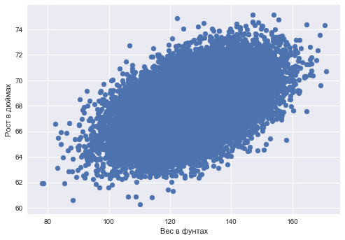
単純なペアワイズ回帰のタスクは、勾配降下法を使用して解決できます。 ある変数を別の変数-体重による成長-を予測し、体重の成長の線形依存性を仮定するとします。
%matplotlib inline from matplotlib import pyplot as plt import seaborn as sns import pandas as pd data_demo = pd.read_csv('../../data/weights_heights.csv')
plt.scatter(data_demo['Weight'], data_demo['Height']); plt.xlabel(' ') plt.ylabel(' ');
ダナベクトル x 長さ ell -各観測(人)の体重値 y -各観測値(人)の成長値のベクトル。
タスク:そのような重みを見つける w0 そして w1 フォームの重量による成長を予測するとき yi=w0+w1xi (どこ yi - i 成長価値 xi - i -th weight of weight)二次誤差を最小化します(可能性があり、平均二乗誤差ですが、定数 frac1 ell 天気はしませんが、 frac12 美のために設立された):
SE(w0、w1)= frac12 sum i=1ell(yi−(w0+w1xi))2\右矢印minw0、w1
関数の偏微分を数える勾配降下の助けを借りてこれを行います SE(w0、w1) モデルの重量で- w0 そして w1 。 反復トレーニング手順は、重みを更新するための簡単な式によって定義されます(小さな、比例的に小さな定数を作成するように重みを変更します) eta 、反勾配機能へのステップ):
beginarrayrclw(t+1)0=w(t)0− eta frac partialSE partialw0|tw(t+1)1=w(t)1− eta frac partialSE partialw1|t endarray
ペンと紙に目を向け、偏微分の分析式を見つけると、次のようになります。
beginarrayrclw(t+1)0=w(t)0+ eta sum elli=1(yi−w(t)0−w(t)1xi)w(t+1)1=w(t)1+ eta sum elli=1(yi−w(t)0−w(t)1xi)xi endarray
そして、これらはすべてうまく機能します(この記事では、極小値の問題、勾配降下ステップの選択、モーメントなどについては説明しません。これについては、多くのことが書かれているので、「Deep Learning」の「数値計算」の章を参照してください)データが多すぎるまで。 このアプローチの問題は、勾配の計算が、トレーニングサンプルの各オブジェクトのいくつかの値の合計に削減されることです。 つまり、問題は、実際にはアルゴリズムの反復には多くの時間が必要であり、各反復でフォームのサンプル全体に合計がある式を使用して重みが再計算されることです sum i=1ell 。 しかし、サンプル内のオブジェクトが数百万と数十億の場合はどうでしょうか?

確率的勾配降下の本質は非公式であり、加重式から合計の符号を捨て、一度に1つのオブジェクトを更新します。 つまり、私たちの場合
beginarrayrclw(t+1)0=w(t)0+ eta(yi−w(t)0−w(t)1xi) w(t+1)1=w(t)1+ eta(yi−w(t)0−w(t)1xi)xi endarray
このアプローチでは、反復ごとに、最速の減少関数への移動がまったく保証されなくなり、通常の勾配降下よりも数桁大きい反復が必要になる場合があります。 ただし、各反復での重みの再計算はほぼ瞬時に行われます。
例として、機械学習コースのAndrew Eunの写真を撮ってください。
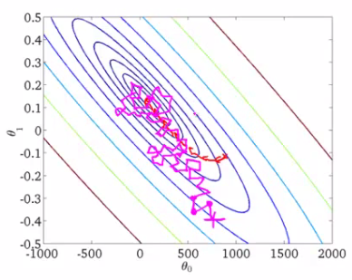
いくつかの関数のレベル線が描かれていますが、これは私たちが探している最小値です。 赤い曲線は、重量の変化を示しています theta0 そして theta1 一致する w0 そして w1 この例では)。 グラデーションのプロパティによると、各ポイントでの変化の方向はレベルラインに垂直になります。 確率論的アプローチでは、各反復で重みの変化が予測しにくく、時にはいくつかのステップが失敗したように見えることもあります-大切な最小値から離れる-しかし、最終的に両方の手順はほぼ同じ解に収束します。
確率的勾配降下法の勾配降下法と同じ解への収束は、最適化理論で証明された最も重要な事実の1つです。 現在、ディープデータとビッグラーニングの時代では、多くの場合、単純に勾配降下法と呼ばれる確率バージョンです。
オンライン学習アプローチ
最適化手法の1つである確率的勾配降下法は、最大数百ギガバイト(使用可能なメモリに依存)の大規模サンプルで分類および回帰アルゴリズムをトレーニングするための非常に実用的なガイドを提供します。
調べたペア回帰の場合、トレーニングセットはディスクに保存できます。 (X、y) そして、RAMにロードせずに(単に収まらない場合があります)、オブジェクトを一度に1つずつ読み取り、重みを更新します。
beginarrayrclw(t+1)0=w(t)0+ eta(yi−w(t)0−w(t)1xi) w(t+1)1=w(t)1+ eta(yi−w(t)0−w(t)1xi)xi endarray
トレーニングサンプルのすべてのオブジェクトを処理した後、最適化する機能(回帰問題の二次誤差、または分類問題のロジスティック誤差など)は減少しますが、多くの場合、サンプルを通過する数十回のパスで十分に減少する必要があります。
モデルトレーニングへのこのアプローチは、オンライン学習と呼ばれることが多く、この用語はMOOCが主流になる前から登場していました。

この記事では、確率的最適化のニュアンスの多くを考慮していません(Habréの良い記事です。このトピックはBoydの本「Convex Optimization」から基本的に学ぶことができます)、Vowpal Wabbitライブラリに移動します。確率的最適化と別のトリック-ハッシュ機能。これについては後で説明します。
Scikit-learn
ライブラリーでは、確率的勾配降下Scikit-learn
分類子とSGDRegressor
は、 SGDClassifier
SGDRegressor
とSGDRegressor
によって実装されます。
カテゴリー機能:ラベルエンコーディング、ワンホットエンコーディング、ハッシュトリック
ラベルのエンコード
分類法と回帰法の大部分は、ユークリッド空間または計量空間に関して定式化されています。つまり、同じ次元の実数ベクトルの形式でデータを表すことを意味します。 ただし、実際のデータでは、yes / noまたは1月/ 2月/.../ 12月などの離散値をとるカテゴリフィーチャはそれほど珍しくありません。 特に線形モデルを使用してこのようなデータを処理する方法、およびカテゴリ属性が多く、それぞれに一意の値が多数ある場合の対処方法について説明します。
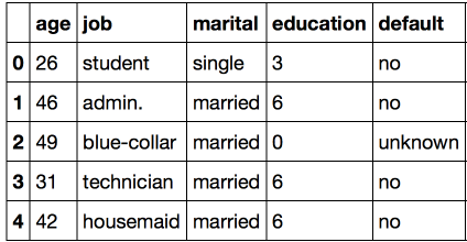
UCI銀行のサンプルを考えてみましょう。ここでは、ほとんどの属性がカテゴリに分類されています。
import warnings warnings.filterwarnings('ignore') import os import re import numpy as np import pandas as pd from sklearn.model_selection import train_test_split from sklearn.linear_model import LogisticRegression from sklearn.metrics import classification_report, accuracy_score from sklearn.metrics import roc_auc_score, roc_curve, confusion_matrix from sklearn.preprocessing import LabelEncoder, OneHotEncoder from sklearn.datasets import fetch_20newsgroups, load_files import pandas as pd from scipy.sparse import csr_matrix import matplotlib.pyplot as plt %matplotlib inline import seaborn as sns df = pd.read_csv('../../data/bank_train.csv') labels = pd.read_csv('../../data/bank_train_target.csv', header=None) df.head()

このデータセットのかなり多くの機能が数字で表されていないことは簡単にわかります。 この形式では、データは依然として私たちに適合していません。利用可能な方法の大部分を使用することはできません。
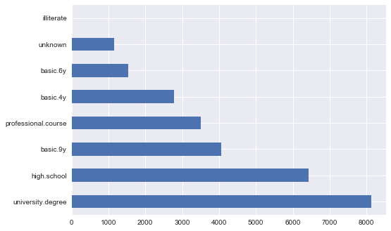
解決策を見つけるために、 education
の兆候を見てみましょう。
df['education'].value_counts().plot.barh();
この問題の自然な解決策は、各値を一意の番号に明確にマッピングすることです。 たとえば、 university.degree
を0に、 basic.9y
を1に変換できます。この単純な操作は頻繁に実行する必要があるため、 sklearn
ライブラリのpreprocessing
モジュールでは、 sklearn
クラスがこのタスクに実装されます。
このクラスのfit
メソッドは、すべての一意の値を検索し、各カテゴリを特定の数値と一致させるテーブルを作成しますtransform
メソッドは、値を直接数値に変換します。 fit
後、 label_encoder
には、すべての一意の値を含むclasses_
フィールドがclasses_
になります。 それらに番号を付け、変換が正しく完了することを確認できます。
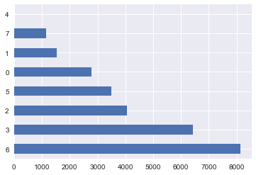
label_encoder = LabelEncoder() mapped_education = pd.Series(label_encoder.fit_transform(df['education'])) mapped_education.value_counts().plot.barh() print(dict(enumerate(label_encoder.classes_)))
{0: 'basic.4y', 1: 'basic.6y', 2: 'basic.9y', 3: 'high.school', 4: 'illiterate', 5: 'professional.course', 6: 'university.degree', 7: 'unknown'}
他のカテゴリのデータがある場合はどうなりますか? LabelEncoder
、新しいカテゴリを知らないとLabelEncoder
ます。
try: label_encoder.transform(df['education'].replace('high.school', 'high_school')) except Exception as e: print('Error:', e)
Error: y contains new labels: ['high_school']
したがって、このアプローチを使用する場合、属性が以前は未知の値をとることができないことを常に確認する必要があります。 少し後でこの問題に戻り、今度はeducation
列全体を変換されたものに置き換えます。
タイプobject
すべての列の変換を続行します。このタイプは、そのようなデータのパンダで指定されます。
categorical_columns = df.columns[df.dtypes == 'object'].union(['education']) for column in categorical_columns: df[column] = label_encoder.fit_transform(df[column]) df.head()
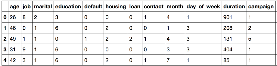
この表現の主な問題は、数値コードがデータのユークリッド表現を作成したことです。
たとえば、仕事の値の上に暗黙的に代数を導入しました-クライアント2の仕事からクライアント1の仕事を差し引くことができます。もちろん、この操作は意味がありません。 しかし、オブジェクトの近接性メトリックが基づいているのはまさにこれに基づいているため、この形式のデータで最近傍法を使用しても意味がありません。 同様に、線形モデルを使用しても意味がありません。 そのようなデータでロジスティック回帰がどのように機能するかを見て、何も良いことが起こらないようにしましょう。
def logistic_regression_accuracy_on(dataframe, labels): features = dataframe.as_matrix() train_features, test_features, train_labels, test_labels = \ train_test_split(features, labels) logit = LogisticRegression() logit.fit(train_features, train_labels) return classification_report(test_labels, logit.predict(test_features)) print(logistic_regression_accuracy_on(df[categorical_columns], labels))
precision recall f1-score support 0 0.89 1.00 0.94 6159 1 0.00 0.00 0.00 740 avg / total 0.80 0.89 0.84 6899
このようなデータで線形モデルを使用できるようにするには、ワンホットエンコードと呼ばれる別の方法が必要です。
ワンホットエンコーディング
特定の特性が10個の異なる値を取ることができると仮定します。 この場合、One Hot Encodingは、1つの例外を除いてすべてがゼロに等しい10個の機能の作成を意味します。 属性の数値に対応する位置に、1を入れます。
この手法は、 OneHotEncoder
クラスのsklearn.preprocessing
で実装されています。 既定では、 OneHotEncoder
、複数のゼロを格納するメモリを無駄にしないように、データをスパース行列に変換します。 ただし、この例では、データサイズは問題ではないため、「高密度」表現を使用します。
onehot_encoder = OneHotEncoder(sparse=False) encoded_categorical_columns = pd.DataFrame(onehot_encoder.fit_transform(df[categorical_columns])) encoded_categorical_columns.head()
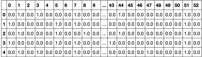
53個の列がありました。これは、元の選択のカテゴリ列で使用できる一意の値の数です。 ワンホットエンコーディングを使用して変換されたデータは、線形モデルに意味があり始めます-クラス1(ローンを確認した人)の精度は61%、充満度)-17%です。
print(logistic_regression_accuracy_on(encoded_categorical_columns, labels))
precision recall f1-score support 0 0.90 0.99 0.94 6126 1 0.61 0.17 0.27 773 avg / total 0.87 0.89 0.87 6899
ハッシュ記号(ハッシュトリック)
実際のデータははるかに動的であることが判明する可能性があり、カテゴリ機能が新しい値をとらないことを常に期待できるわけではありません。 これはすべて、新しいデータで既に訓練されたモデルの使用を非常に複雑にします。 さらに、 LabelEncoder
では、サンプル全体の予備分析と、構築されたマッピングのメモリへの保存が行われるため、ビッグデータモードでの作業が困難になります。
これらの問題を解決するために、ハッシュトリックとして知られるハッシュに基づいて、カテゴリフィーチャをハッシュするより簡単なアプローチがあります。
ハッシュ関数は、次のようなさまざまな属性値の一意のコードを見つけるタスクで役立ちます。
for s in ('university.degree', 'high.school', 'illiterate'): print(s, '->', hash(s))
university.degree -> -5073140156977989958 high.school -> -8439808450962279468 illiterate -> -2719819637717010547
負の非常に大きなモジュロ値は適切ではありません。 ハッシュ関数の値の範囲を制限します。
hash_space = 25 for s in ('university.degree', 'high.school', 'illiterate'): print(s, '->', hash(s) % hash_space)
university.degree -> 17 high.school -> 7 illiterate -> 3
サンプルに1人の学生が月曜日に呼び出され、彼の特徴ベクトルがOne-Hot Encodingと同様に形成されますが、すべての特徴に対して固定サイズの単一のスペースにあるとします。
hashing_example = pd.DataFrame([{i: 0.0 for i in range(hash_space)}]) for s in ('job=student', 'marital=single', 'day_of_week=mon'): print(s, '->', hash(s) % hash_space) hashing_example.loc[0, hash(s) % hash_space] = 1 hashing_example
job=student -> 6 marital=single -> 8 day_of_week=mon -> 16
この例では、属性の値がハッシュされただけでなく、 属性名と属性値のペアがハッシュされたことに注意してください。 これは、たとえば以下のように、異なる特性の同じ値を共有するために必要です。
assert hash('no') == hash('no') assert hash('housing=no') != hash('loan=no')
ハッシュ関数は衝突できますか?つまり、2つの異なる値のコード間の一致ですか? 十分な量のハッシュ空間ではこれはめったに起こらないことを証明するのは簡単ですが、これが起こる場合でも、分類または回帰の品質の著しい低下につながらないでしょう。

「一体何が起こっているのか?」と尋ねることができます。また、属性をハッシュする際に常識が損なわれているように見えます。 おそらく、しかし、この経験則は、実際には、多くのユニークな意味を持つカテゴリ属性を操作するための唯一のアプローチです。 さらに、この手法は実際的な結果の点で実証されています。 このレビューと Evgeny Sokolovの資料で、ハッシュ記号(ハッシュの学習)について詳しく読むことができます。
Vowpal Wabbit Library
Vowpal Wabbit(VW)は、業界で最も広く使用されているライブラリの1つです。 高速性と多数の異なるトレーニングモードのサポートを特長としています。 大規模で高次元のデータにとって特に興味深いのは、図書館の最大の強みであるオンライン学習です。 機能ハッシュも実装されており、Vowpal Wabbitはテキストデータの操作に最適です。
VWを操作するためのメインインターフェイスはシェルです。 Vowpal Wabbitは、次のような形式でファイルまたは標準入力(stdin)からデータを読み取ります。
[Label] [Importance] [Tag]|Namespace Features |Namespace Features ... |Namespace Features
Namespace=String[:Value]
Features=(String[:Value] )*
ここで、[]はオプションの要素を示し、(...)*は無制限の回数の繰り返しを意味します。
- ラベルは数字であり、「正しい」答えです。 分類の場合、通常は1 / -1の値を取り、回帰の場合、実数
- 重要度は数値であり、トレーニングの例の重みに責任があります。 これにより、以前に調査した不均衡なデータの問題に対処できます。
- タグはスペースを含まない文字列で、応答の予測時に保存される例の「名前」の一部を担います。 重要度からタグを分離するには、「文字」でタグを開始することをお勧めします。
- 名前空間は、個別の機能空間を作成するために使用されます。 名前空間の引数は最初の文字で名前が付けられます。名前を選択する際にはこれを考慮する必要があります
- 機能は、 名前空間内のオブジェクトの属性です。 記号のデフォルトの重みは1.0ですが、feature:0.1のようにオーバーライドできます。
たとえば、次の行はこのような形式に適しています。
1 1.0 |Subject WHAT car is this |Organization University of Maryland:0.5 College Park
VWは、テキストデータを操作するための優れたツールです。 20件のさまざまな件名のメールからのニュースを含む20件のニュースグループを選択することで、それを確信します。
ニュース。 バイナリ分類
newsgroups = fetch_20newsgroups('../../data/news_data')
各ニュース項目は、alt.atheism、comp.graphics、comp.os.ms-windows.misc、comp.sys.ibm.pc.hardware、comp.sys.mac.hardware、comp.windows.xの20のトピックのいずれかに関連しています。 、misc.forsalerec.autos、rec.motorcycles、rec.sport.baseball、rec.sport.hockey、sci.crypt、sci.electronics、sci.med、sci.space、soc.religion.christian、talk.politics.guns 、talk.politics.mideast、talk.politics.misc、talk.religion.misc。
このコレクションの最初のテキストドキュメントを考えてみましょう。
text = newsgroups['data'][0] target = newsgroups['target_names'][newsgroups['target'][0]] print('-----') print(target) print('-----') print(text.strip()) print('----')
----- rec.autos ----- From: lerxst@wam.umd.edu (where's my thing) Subject: WHAT car is this!? Nntp-Posting-Host: rac3.wam.umd.edu Organization: University of Maryland, College Park Lines: 15 I was wondering if anyone out there could enlighten me on this car I saw the other day. It was a 2-door sports car, looked to be from the late 60s/ early 70s. It was called a Bricklin. The doors were really small. In addition, the front bumper was separate from the rest of the body. This is all I know. If anyone can tellme a model name, engine specs, years of production, where this car is made, history, or whatever info you have on this funky looking car, please e-mail. Thanks, - IL ---- brought to you by your neighborhood Lerxst ---- ----
データをVowpal Wabbit形式に変換し、3文字以上の単語のみを残しましょう。 ここでは、テキストの分析(ステミングおよび見出し語化)で多くの重要な手順を実行しませんが、後で説明するように、タスクはとにかく解決されます。
def to_vw_format(document, label=None): return str(label or '') + ' |text ' + ' '.join(re.findall('\w{3,}', document.lower())) + '\n' to_vw_format(text, 1 if target == 'rec.autos' else -1)
'1 |text from lerxst wam umd edu where thing subject what car this nntp posting host rac3 wam umd edu organization university maryland college park lines was wondering anyone out there could enlighten this car saw the other day was door sports car looked from the late 60s early 70s was called bricklin the doors were really small addition the front bumper was separate from the rest the body this all know anyone can tellme model name engine specs years production where this car made history whatever info you have this funky looking car please mail thanks brought you your neighborhood lerxst\n'
サンプルをトレーニングとテストに分け、ドキュメントをファイルに変換します。 それが自動車rec.autosについてのニュースレターに関連しているならば、我々は文書をポジティブと考えます。 そこで、自動車に関するニュースとその他のニュースを区別するモデルを構築します。
all_documents = newsgroups['data'] all_targets = [1 if newsgroups['target_names'][target] == 'rec.autos' else -1 for target in newsgroups['target']]
train_documents, test_documents, train_labels, test_labels = \ train_test_split(all_documents, all_targets, random_state=7) with open('../../data/news_data/20news_train.vw', 'w') as vw_train_data: for text, target in zip(train_documents, train_labels): vw_train_data.write(to_vw_format(text, target)) with open('../../data/news_data/20news_test.vw', 'w') as vw_test_data: for text in test_documents: vw_test_data.write(to_vw_format(text))
生成されたファイルでVowpal Wabbitを実行します。 分類問題を解決するため、損失関数をヒンジ(線形SVM)に設定します。 作成したモデルを対応するファイル20news_model.vw
保存します。
!vw -d ../../data/news_data/20news_train.vw \ --loss_function hinge -f ../../data/news_data/20news_model.vw
final_regressor = ../../data/news_data/20news_model.vw Num weight bits = 18 learning rate = 0.5 initial_t = 0 power_t = 0.5 using no cache Reading datafile = ../../data/news_data/20news_train.vw num sources = 1 average since example example current current current loss last counter weight label predict features 1.000000 1.000000 1 1.0 -1.0000 0.0000 157 0.911276 0.822551 2 2.0 -1.0000 -0.1774 159 0.605793 0.300311 4 4.0 -1.0000 -0.3994 92 0.419594 0.233394 8 8.0 -1.0000 -0.8167 129 0.313998 0.208402 16 16.0 -1.0000 -0.6509 108 0.196014 0.078029 32 32.0 -1.0000 -1.0000 115 0.183158 0.170302 64 64.0 -1.0000 -0.7072 114 0.261046 0.338935 128 128.0 1.0000 -0.7900 110 0.262910 0.264774 256 256.0 -1.0000 -0.6425 44 0.216663 0.170415 512 512.0 -1.0000 -1.0000 160 0.176710 0.136757 1024 1024.0 -1.0000 -1.0000 194 0.134541 0.092371 2048 2048.0 -1.0000 -1.0000 438 0.104403 0.074266 4096 4096.0 -1.0000 -1.0000 644 0.081329 0.058255 8192 8192.0 -1.0000 -1.0000 174 finished run number of examples per pass = 8485 passes used = 1 weighted example sum = 8485.000000 weighted label sum = -7555.000000 average loss = 0.079837 best constant = -1.000000 best constant's loss = 0.109605 total feature number = 2048932
モデルは訓練されています。 VWは、トレーニング中に非常に多くの有用な情報を表示します(それでも、-quietパラメーターを設定することにより、返済できます)。 診断情報の詳細な出力は、GitHubのVWドキュメントで分析されます( こちら) 。 反復中に平均損失が減少したことに注意してください。 損失関数を計算するために、VWはまだ表示されていない例を使用します。したがって、原則として、この推定は正しいです。 訓練されたモデルをテストセットに適用し、-pオプションを使用して予測をファイルに保存します。
!vw -i ../../data/news_data/20news_model.vw -t -d ../../data/news_data/20news_test.vw \ -p ../../data/news_data/20news_test_predictions.txt
only testing predictions = ../../data/news_data/20news_test_predictions.txt Num weight bits = 18 learning rate = 0.5 initial_t = 0 power_t = 0.5 using no cache Reading datafile = ../../data/news_data/20news_test.vw num sources = 1 average since example example current current current loss last counter weight label predict features 0.000000 0.000000 1 1.0 unknown 1.0000 349 0.000000 0.000000 2 2.0 unknown -1.0000 50 0.000000 0.000000 4 4.0 unknown -1.0000 251 0.000000 0.000000 8 8.0 unknown -1.0000 237 0.000000 0.000000 16 16.0 unknown -0.8978 106 0.000000 0.000000 32 32.0 unknown -1.0000 964 0.000000 0.000000 64 64.0 unknown -1.0000 261 0.000000 0.000000 128 128.0 unknown 0.4621 82 0.000000 0.000000 256 256.0 unknown -1.0000 186 0.000000 0.000000 512 512.0 unknown -1.0000 162 0.000000 0.000000 1024 1024.0 unknown -1.0000 283 0.000000 0.000000 2048 2048.0 unknown -1.0000 104 finished run number of examples per pass = 2829 passes used = 1 weighted example sum = 2829.000000 weighted label sum = 0.000000 average loss = 0.000000 total feature number = 642215
, AUC ROC-:
with open('../../data/news_data/20news_test_predictions.txt') as pred_file: test_prediction = [float(label) for label in pred_file.readlines()] auc = roc_auc_score(test_labels, test_prediction) roc_curve = roc_curve(test_labels, test_prediction) with plt.xkcd(): plt.plot(roc_curve[0], roc_curve[1]); plt.plot([0,1], [0,1]) plt.xlabel('FPR'); plt.ylabel('TPR'); plt.title('test AUC = %f' % (auc)); plt.axis([-0.05,1.05,-0.05,1.05]);
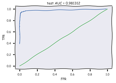
AUC .
.
, , . Vowpal Wabbit
– , 1 K, K – ( – 20). LabelEncoder, ( LabelEncoder
0 K-1).
all_documents = newsgroups['data'] topic_encoder = LabelEncoder() all_targets_mult = topic_encoder.fit_transform(newsgroups['target']) + 1
, , train_labels_mult
test_labels_mult
– 1 20.
train_documents, test_documents, train_labels_mult, test_labels_mult = \ train_test_split(all_documents, all_targets_mult, random_state=7) with open('../../data/news_data/20news_train_mult.vw', 'w') as vw_train_data: for text, target in zip(train_documents, train_labels_mult): vw_train_data.write(to_vw_format(text, target)) with open('../../data/news_data/20news_test_mult.vw', 'w') as vw_test_data: for text in test_documents: vw_test_data.write(to_vw_format(text))
Vowpal Wabbit , oaa
( "one against all"), . , , ( – Vowpal Wabbit):
- (-l, 0.5) –
- (--power_t, 0.5) – , ,
- (--loss_function) – , , .
(-l1) – , VW , , 10−20.
Vowpal Wabbit Hyperopt. Python 2. .
%%time !vw --oaa 20 ../../data/news_data/20news_train_mult.vw \ -f ../../data/news_data/20news_model_mult.vw --loss_function=hinge
final_regressor = ../../data/news_data/20news_model_mult.vw Num weight bits = 18 learning rate = 0.5 initial_t = 0 power_t = 0.5 using no cache Reading datafile = ../../data/news_data/20news_train_mult.vw num sources = 1 average since example example current current current loss last counter weight label predict features 1.000000 1.000000 1 1.0 15 1 157 1.000000 1.000000 2 2.0 2 15 159 1.000000 1.000000 4 4.0 15 10 92 1.000000 1.000000 8 8.0 16 15 129 1.000000 1.000000 16 16.0 13 12 108 0.937500 0.875000 32 32.0 2 9 115 0.906250 0.875000 64 64.0 16 16 114 0.867188 0.828125 128 128.0 8 4 110 0.816406 0.765625 256 256.0 7 15 44 0.646484 0.476562 512 512.0 13 9 160 0.502930 0.359375 1024 1024.0 3 4 194 0.388672 0.274414 2048 2048.0 1 1 438 0.300293 0.211914 4096 4096.0 11 11 644 0.225098 0.149902 8192 8192.0 5 5 174 finished run number of examples per pass = 8485 passes used = 1 weighted example sum = 8485.000000 weighted label sum = 0.000000 average loss = 0.222392 total feature number = 2048932 CPU times: user 7.97 ms, sys: 13.9 ms, total: 21.9 ms Wall time: 378 ms
%%time !vw -i ../../data/news_data/20news_model_mult.vw -t \ -d ../../data/news_data/20news_test_mult.vw \ -p ../../data/news_data/20news_test_predictions_mult.txt
only testing predictions = ../../data/news_data/20news_test_predictions_mult.txt Num weight bits = 18 learning rate = 0.5 initial_t = 0 power_t = 0.5 using no cache Reading datafile = ../../data/news_data/20news_test_mult.vw num sources = 1 average since example example current current current loss last counter weight label predict features 1.000000 1.000000 1 1.0 unknown 8 349 1.000000 1.000000 2 2.0 unknown 6 50 1.000000 1.000000 4 4.0 unknown 18 251 1.000000 1.000000 8 8.0 unknown 18 237 1.000000 1.000000 16 16.0 unknown 4 106 1.000000 1.000000 32 32.0 unknown 15 964 1.000000 1.000000 64 64.0 unknown 4 261 1.000000 1.000000 128 128.0 unknown 8 82 1.000000 1.000000 256 256.0 unknown 10 186 1.000000 1.000000 512 512.0 unknown 1 162 1.000000 1.000000 1024 1024.0 unknown 11 283 1.000000 1.000000 2048 2048.0 unknown 14 104 finished run number of examples per pass = 2829 passes used = 1 weighted example sum = 2829.000000 weighted label sum = 0.000000 average loss = 1.000000 total feature number = 642215 CPU times: user 4.28 ms, sys: 9.65 ms, total: 13.9 ms Wall time: 166 ms
with open('../../data/news_data/20news_test_predictions_mult.txt') as pred_file: test_prediction_mult = [float(label) for label in pred_file.readlines()]
accuracy_score(test_labels_mult, test_prediction_mult)
87%.
, , .
M = confusion_matrix(test_labels_mult, test_prediction_mult) for i in np.where(M[0,:] > 0)[0][1:]: print(newsgroups['target_names'][i], M[0,i], )
rec.autos 1 rec.sport.baseball 1 sci.med 1 soc.religion.christian 3 talk.religion.misc 5
: rec.autos, rec.sport.baseball, sci.med, soc.religion.christian talk.religion.misc.
IMDB
, IMDB. , Vowpal Wabbit.
load_files
sklearn.datasets
. imdb_reviews
( train test ). – 100 . . 12500 . (, ) .
# path_to_movies = '/Users/y.kashnitsky/Yandex.Disk.localized/ML/data/imdb_reviews/' reviews_train = load_files(os.path.join(path_to_movies, 'train')) text_train, y_train = reviews_train.data, reviews_train.target
print("Number of documents in training data: %d" % len(text_train)) print(np.bincount(y_train))
Number of documents in training data: 25000 [12500 12500]
.
reviews_test = load_files(os.path.join(path_to_movies, 'test')) text_test, y_test = reviews_test.data, reviews_train.target print("Number of documents in test data: %d" % len(text_test)) print(np.bincount(y_test))
Number of documents in test data: 25000 [12500 12500]
:
"Zero Day leads you to think, even re-think why two boys/young men would do what they did - commit mutual suicide via slaughtering their classmates. It captures what must be beyond a bizarre mode of being for two humans who have decided to withdraw from common civility in order to define their own/mutual world via coupled destruction.<br /><br />It is not a perfect movie but given what money/time the filmmaker and actors had - it is a remarkable product. In terms of explaining the motives and actions of the two young suicide/murderers it is better than 'Elephant' - in terms of being a film that gets under our 'rationalistic' skin it is a far, far better film than almost anything you are likely to see. <br /><br />Flawed but honest with a terrible honesty."
. :
'Words can\'t describe how bad this movie is. I can\'t explain it by writing only. You have too see it for yourself to get at grip of how horrible a movie really can be. Not that I recommend you to do that. There are so many clich\xc3\xa9s, mistakes (and all other negative things you can imagine) here that will just make you cry. To start with the technical first, there are a LOT of mistakes regarding the airplane. I won\'t list them here, but just mention the coloring of the plane. They didn\'t even manage to show an airliner in the colors of a fictional airline, but instead used a 747 painted in the original Boeing livery. Very bad. The plot is stupid and has been done many times before, only much, much better. There are so many ridiculous moments here that i lost count of it really early. Also, I was on the bad guys\' side all the time in the movie, because the good guys were so stupid. "Executive Decision" should without a doubt be you\'re choice over this one, even the "Turbulence"-movies are better. In fact, every other movie in the world is better than this one.'
to_vw_format
. ( movie_reviews_train.vw
), ( movie_reviews_valid.vw
) ( movie_reviews_test.vw
) Vowpal Wabbit. 70% , 30% – .
train_share = int(0.7 * len(text_train)) train, valid = text_train[:train_share], text_train[train_share:] train_labels, valid_labels = y_train[:train_share], y_train[train_share:] with open('../../data/movie_reviews_train.vw', 'w') as vw_train_data: for text, target in zip(train, train_labels): vw_train_data.write(to_vw_format(str(text), 1 if target == 1 else -1)) with open('../../data/movie_reviews_valid.vw', 'w') as vw_train_data: for text, target in zip(valid, valid_labels): vw_train_data.write(to_vw_format(str(text), 1 if target == 1 else -1)) with open('../../data/movie_reviews_test.vw', 'w') as vw_test_data: for text in text_test: vw_test_data.write(to_vw_format(str(text)))
Vowpal Wabbit :
- -d, (. .vw )
- --loss_function – hinge ( )
- -f – , ( .vw)
!vw -d ../../data/movie_reviews_train.vw \ --loss_function hinge -f movie_reviews_model.vw --quiet
Vowpal Wabbit, :
- -i – (. .vw)
- -t -d – (. .vw)
- -p – txt-,
!vw -i movie_reviews_model.vw -t -d ../../data/movie_reviews_valid.vw \ -p movie_valid_pred.txt --quiet
ROC AUC. , VW +1. [-1, 1], (0 1) , . AUC 88.5% – 94.2% – .
with open('movie_valid_pred.txt') as pred_file: valid_prediction = [float(label) for label in pred_file.readlines()] print("Accuracy: {}".format(round(accuracy_score(valid_labels, [int(pred_prob > 0) for pred_prob in valid_prediction]), 3))) print("AUC: {}".format(round(roc_auc_score(valid_labels, valid_prediction), 3)))
!vw -i movie_reviews_model.vw -t -d ../../data/movie_reviews_test.vw \ -p movie_test_pred.txt --quiet
with open('movie_test_pred.txt') as pred_file: test_prediction = [float(label) for label in pred_file.readlines()] print("Accuracy: {}".format(round(accuracy_score(y_test, [int(pred_prob > 0) for pred_prob in test_prediction]), 3))) print("AUC: {}".format(round(roc_auc_score(y_test, test_prediction), 3)))
Accuracy: 0.88 AUC: 0.94
. – 89% AUC 95% .
!vw -d ../../data/movie_reviews_train.vw \ --loss_function hinge --ngram 2 -f movie_reviews_model2.vw --quiet
!vw -i movie_reviews_model2.vw -t -d ../../data/movie_reviews_valid.vw \ -p movie_valid_pred2.txt --quiet
with open('movie_valid_pred2.txt') as pred_file: valid_prediction = [float(label) for label in pred_file.readlines()] print("Accuracy: {}".format(round(accuracy_score(valid_labels, [int(pred_prob > 0) for pred_prob in valid_prediction]), 3))) print("AUC: {}".format(round(roc_auc_score(valid_labels, valid_prediction), 3)))
Accuracy: 0.894 AUC: 0.954
!vw -i movie_reviews_model2.vw -t -d ../../data/movie_reviews_test.vw \ -p movie_test_pred2.txt --quiet
with open('movie_test_pred2.txt') as pred_file: test_prediction2 = [float(label) for label in pred_file.readlines()] print("Accuracy: {}".format(round(accuracy_score(y_test, [int(pred_prob > 0) for pred_prob in test_prediction2]), 3))) print("AUC: {}".format(round(roc_auc_score(y_test, test_prediction2), 3)))
Accuracy: 0.888 AUC: 0.952
StackOverflow
, Vowpal Wabbit . 10 StackOverflow – , 10 , . , .

10, 10 : 10 , 10 .
# PATH_TO_DATA = '/Users/y.kashnitsky/Documents/Machine_learning/org_mlcourse_ai/private/stackoverflow_hw/' !du -hs $PATH_TO_DATA/stackoverflow_10mln_*.vw
1,4G /Users/y.kashnitsky/Documents/Machine_learning/org_mlcourse_ai/private/stackoverflow_hw//stackoverflow_10mln_test.vw 3,3G /Users/y.kashnitsky/Documents/Machine_learning/org_mlcourse_ai/private/stackoverflow_hw//stackoverflow_10mln_train.vw 1,9G /Users/y.kashnitsky/Documents/Machine_learning/org_mlcourse_ai/private/stackoverflow_hw//stackoverflow_10mln_train_part.vw 1,4G /Users/y.kashnitsky/Documents/Machine_learning/org_mlcourse_ai/private/stackoverflow_hw//stackoverflow_10mln_valid.vw
, Vowpal Wabbit. 10 10 , .
10 | i ve got some code in window scroll that checks if an element is visible then triggers another function however only the first section of code is firing both bits of code work in and of themselves if i swap their order whichever is on top fires correctly my code is as follows fn isonscreen function use strict var win window viewport top win scrolltop left win scrollleft bounds this offset viewport right viewport left + win width viewport bottom viewport top + win height bounds right bounds left + this outerwidth bounds bottom bounds top + this outerheight return viewport right lt bounds left viewport left gt bounds right viewport bottom lt bounds top viewport top gt bounds bottom window scroll function use strict var load_more_results ajax load_more_results isonscreen if load_more_results true loadmoreresults var load_more_staff ajax load_more_staff isonscreen if load_more_staff true loadmorestaff what am i doing wrong can you only fire one event from window scroll i assume not
(3.3 ) Vowpal Wabbit :
- -oaa 10 – , 10
- -d –
- -f – ,
- -b 28 – 28 , 228 , , ( - , )
- random seed
%%time !vw --oaa 10 -d $PATH_TO_DATA/stackoverflow_10mln_train.vw \ -f vw_model1_10mln.vw -b 28 --random_seed 17 --quiet
CPU times: user 592 ms, sys: 220 ms, total: 813 ms Wall time: 39.9 s
40 , 14 , – 92%. , . .
%%time !vw -t -i vw_model1_10mln.vw \ -d $PATH_TO_DATA/stackoverflow_10mln_test.vw \ -p vw_valid_10mln_pred1.csv --random_seed 17 --quiet
CPU times: user 198 ms, sys: 83.1 ms, total: 281 ms Wall time: 14.1 s
import os import numpy as np from sklearn.metrics import accuracy_score vw_pred = np.loadtxt('vw_valid_10mln_pred1.csv') test_labels = np.loadtxt(os.path.join(PATH_TO_DATA, 'stackoverflow_10mln_test_labels.txt')) accuracy_score(test_labels, vw_pred)
0.91868709729356979
宿題
- . Jupyter notebook - ( ).
便利なリンク
- Open Machine Learning Course. Topic 8. Vowpal Wabbit: Fast Learning with Gigabytes of Data
- : ( ), ( ), Vowpal Wabbit
- "Numeric Computation" "Deep Learning"
- Vowpal Wabbit GitHub
- , (VW) Hadoop-
- VW
- VW hyperopt
Jupyter GitHub- .