👩‍❤️‍👨 💠 🦅 データサイエンスで1か月に大量にポンプを使用する方法 👨🏽‍🚒 🕢 📬

こんにちは、Habr！

私の名前はGlebです。長い間小売分析に取り組んでおり、現在この分野で機械学習の使用に携わっています。少し前のことですが、 MLClass.ruのメンバーに会いました。彼は非常に短期間で、 データサイエンスの分野で私をかなり励ましました。彼らのおかげで、たった一ヶ月で私は積極的にkaggleに応募し始めました。したがって、この一連の出版物では、データサイエンスの研究における私の経験、犯したすべての間違い、そして彼らからの貴重なアドバイスについて説明します。今日は、 Analytics Edgeコンペティション（2015年春）に参加した経験についてお話します。これは私の最初の記事です-厳密に判断しないでください。

説明されたコンペティションは、「マサチューセッツ工科大学」のコース「アナリティクスエッジ」の一部として開催されました。以下で、 Rの言語でコードを提供します。

タスクの説明

販売者は、製品のどの特性が製品を販売する可能性を高めるかを知りたいと考えています。この競争では、 eBay Webサイトから取得したデータに基づいてApple iPadが販売される可能性を予測するモデルを調査することが提案されました。

データ

研究用に提案されたデータは、2つのファイルで構成されていました。

eBayiPadTrain.csv-モデルを作成するためのデータセット。 1861個のアイテムが含まれています。
eBayiPadTest.csv-モデルを評価するためのデータ

開始するには、作業で使用されるライブラリを接続します。

library(dplyr) #      library(readr) #

データをロードします。

 eBayTrain <- read_csv("eBayiPadTrain.csv") eBayTest <- read_csv("eBayiPadTest.csv")

データ構造を見てみましょう。

 summary(eBayTrain) ## description biddable startprice condition ## Length:1861 Min. :0.0000 Min. : 0.01 Length:1861 ## Class :character 1st Qu.:0.0000 1st Qu.: 80.00 Class :character ## Mode :character Median :0.0000 Median :179.99 Mode :character ## Mean :0.4498 Mean :211.18 ## 3rd Qu.:1.0000 3rd Qu.:300.00 ## Max. :1.0000 Max. :999.00 ## cellular carrier color ## Length:1861 Length:1861 Length:1861 ## Class :character Class :character Class :character ## Mode :character Mode :character Mode :character ## ## ## ## storage productline sold UniqueID ## Length:1861 Length:1861 Min. :0.0000 Min. :10001 ## Class :character Class :character 1st Qu.:0.0000 1st Qu.:10466 ## Mode :character Mode :character Median :0.0000 Median :10931 ## Mean :0.4621 Mean :10931 ## 3rd Qu.:1.0000 3rd Qu.:11396 ## Max. :1.0000 Max. :11861 str(eBayTrain) ## Classes 'tbl_df', 'tbl' and 'data.frame': 1861 obs. of 11 variables: ## $ description: chr "iPad is in 8.5+ out of 10 cosmetic condition!" "Previously used, please read description. May show signs of use such as scratches to the screen and " "" "" ... ## $ biddable : int 0 1 0 0 0 1 1 0 1 1 ... ## $ startprice : num 159.99 0.99 199.99 235 199.99 ... ## $ condition : chr "Used" "Used" "Used" "New other (see details)" ... ## $ cellular : chr "0" "1" "0" "0" ... ## $ carrier : chr "None" "Verizon" "None" "None" ... ## $ color : chr "Black" "Unknown" "White" "Unknown" ... ## $ storage : chr "16" "16" "16" "16" ... ## $ productline: chr "iPad 2" "iPad 2" "iPad 4" "iPad mini 2" ... ## $ sold : int 0 1 1 0 0 1 1 0 1 1 ... ## $ UniqueID : int 10001 10002 10003 10004 10005 10006 10007 10008 10009 10010 ...

データセットは11の変数で構成されています。

description-売り手が提供した商品の説明文
入札可能 -アイテムはオークションにかけられます（= 1）または固定価格（= 0）で
startprice-オークションの開始価格（入札可能 = 1の場合）または販売価格（ 入札可能 = 0の場合）
状態 -商品の状態（新品、中古品など）
セルラー -モバイル通信のある製品（= 1）またはそうでない（= 0）
キャリア -キャリア（ セルラー = 1の場合）
色 -色
ストレージ -メモリサイズ
製品ライン -製品モデル名
sold-製品が販売されたか（= 1）否か（= 0）。これは従属変数になります。
UniqueID-一意のシリアル番号

したがって、3種類の変数があります：テキストの説明、数値の開始価格、およびその他のすべては階乗です。

追加の変数を作成する

商品のどの部分に説明があるか見てみましょう

 table(eBayTrain$description == "") ## ## FALSE TRUE ## 790 1071

すべての製品に説明があるわけではないので、このパラメーターが販売の可能性に影響する可能性があることを提案しました。これを考慮するために、説明があれば値1を、そうでなければ0をとる変数を作成します。

 eBayTrain$is_descr = as.factor(eBayTrain$description == "") table(eBayTrain$description == "", eBayTrain$is_descr) ## ## FALSE TRUE ## FALSE 790 0 ## TRUE 0 1071

テキスト記述からモデルの変数を作成する

テキストの説明に基づいて、頻繁に発生する単語を強調表示して、モデルの変数を作成します。これを行うには、 tmライブラリを使用します。

 library(tm) ##   ## Loading required package: NLP ##    ,     CorpusDescription <- Corpus(VectorSource(c(eBayTrain$description, eBayTest$description))) ##      CorpusDescription <- tm_map(CorpusDescription, content_transformer(tolower)) CorpusDescription <- tm_map(CorpusDescription, PlainTextDocument) ##    CorpusDescription <- tm_map(CorpusDescription, removePunctuation) ##    -, .. ,     CorpusDescription <- tm_map(CorpusDescription, removeWords, stopwords("english")) ##  , ..      CorpusDescription <- tm_map(CorpusDescription, stemDocument) ##    dtm <- DocumentTermMatrix(CorpusDescription) ##    sparse <- removeSparseTerms(dtm, 0.97) ##     data.frame       DescriptionWords = as.data.frame(as.matrix(sparse)) colnames(DescriptionWords) = make.names(colnames(DescriptionWords)) DescriptionWordsTrain = head(DescriptionWords, nrow(eBayTrain)) DescriptionWordsTest = tail(DescriptionWords, nrow(eBayTest))

次に、残りのテキスト変数をファクターデータ型に変換して、モデルがそれらをテキストとして処理しないようにします。そして、それらを製品の説明から取得した変数と組み合わせます。このために、非常に便利なmagnittrライブラリを使用します

 library(magrittr) eBayTrain %<>% mutate(condition = as.factor(condition), cellular = as.factor(cellular), carrier = as.factor(carrier), color = as.factor(color), storage = as.factor(storage), productline = as.factor(productline), sold = as.factor(sold)) %>% select(-description, -UniqueID ) %>% cbind(., DescriptionWordsTrain)

結果の変数セットを見てみましょう。

 str(eBayTrain) ## 'data.frame': 1861 obs. of 30 variables: ## $ biddable : int 0 1 0 0 0 1 1 0 1 1 ... ## $ startprice : num 159.99 0.99 199.99 235 199.99 ... ## $ condition : Factor w/ 6 levels "For parts or not working",..: 6 6 6 4 5 6 3 3 6 6 ... ## $ cellular : Factor w/ 3 levels "0","1","Unknown": 1 2 1 1 3 2 1 1 2 1 ... ## $ carrier : Factor w/ 7 levels "AT&T","None",..: 2 7 2 2 6 1 2 2 6 2 ... ## $ color : Factor w/ 5 levels "Black","Gold",..: 1 4 5 4 4 3 3 5 5 5 ... ## $ storage : Factor w/ 5 levels "128","16","32",..: 2 2 2 2 5 3 2 2 4 3 ... ## $ productline: Factor w/ 12 levels "iPad 1","iPad 2",..: 2 2 4 9 12 9 8 10 1 4 ... ## $ sold : Factor w/ 2 levels "0","1": 1 2 2 1 1 2 2 1 2 2 ... ## $ is_descr : Factor w/ 2 levels "FALSE","TRUE": 1 1 2 2 1 2 2 2 2 2 ... ## $ box : num 0 0 0 0 0 0 0 0 0 0 ... ## $ condit : num 1 0 0 0 0 0 0 0 0 0 ... ## $ cosmet : num 1 0 0 0 0 0 0 0 0 0 ... ## $ devic : num 0 0 0 0 0 0 0 0 0 0 ... ## $ excel : num 0 0 0 0 0 0 0 0 0 0 ... ## $ fulli : num 0 0 0 0 0 0 0 0 0 0 ... ## $ function. : num 0 0 0 0 0 0 0 0 0 0 ... ## $ good : num 0 0 0 0 0 0 0 0 0 0 ... ## $ great : num 0 0 0 0 0 0 0 0 0 0 ... ## $ includ : num 0 0 0 0 0 0 0 0 0 0 ... ## $ ipad : num 1 0 0 0 0 0 0 0 0 0 ... ## $ item : num 0 0 0 0 0 0 0 0 0 0 ... ## $ light : num 0 0 0 0 0 0 0 0 0 0 ... ## $ minor : num 0 0 0 0 0 0 0 0 0 0 ... ## $ new : num 0 0 0 0 0 0 0 0 0 0 ... ## $ scratch : num 0 1 0 0 0 0 0 0 0 0 ... ## $ screen : num 0 1 0 0 0 0 0 0 0 0 ... ## $ use : num 0 2 0 0 0 0 0 0 0 0 ... ## $ wear : num 0 0 0 0 0 0 0 0 0 0 ... ## $ work : num 0 0 0 0 0 0 0 0 0 0 ...

他の変数と比較して値の範囲がはるかに広いため、この変数がモデルの結果に過度の影響を与えないように、 startprice変数を正規化します。

 eBayTrain$startprice <- (eBayTrain$startprice - mean(eBayTrain$startprice))/sd(eBayTrain$startprice)

モデル

結果のデータセットを使用して、モデルを作成します。モデルの評価の正確性を評価するために、競争で選択されたものと同じ評価を適用します。これはAUCです。このパラメーターは、分類モデルの評価によく使用されます。これは、モデルがランダムデータセットから従属変数を正しく決定する確率を反映しています。理想的なモデルでは、 AUCが1.0に等しく、ランダムに推測される確率が同等のモデル-0.5が表示されます。

競争の形式は1日1回の限られた回数であり、結果をウェブサイトにアップロードして取得したモデルを検証するために使用できるため、トレーニングデータセットから独自のテストサンプルを選択してモデルを評価します。バランスの取れたサンプルを取得するには、 caToolsライブラリを使用します。

 set.seed(1000) ##    library(caTools) split <- sample.split(eBayTrain$sold, SplitRatio = 0.7) train <- filter(eBayTrain, split == T) test <- filter(eBayTrain, split == F)

ロジスティック分類

ロジスティック回帰モデルを作成する

 model_glm1 <- glm(sold ~ ., data = train, family = binomial)

モデルの変数の重要性を見てみましょう。

 summary(model_glm1) ## ## Call: ## glm(formula = sold ~ ., family = binomial, data = train) ## ## Deviance Residuals: ## Min 1Q Median 3Q Max ## -2.6620 -0.7308 -0.2450 0.6229 3.5600 ## ## Coefficients: ## Estimate Std. Error z value Pr(>|z|) ## (Intercept) 11.91318 619.41930 0.019 0.984655 ## biddable 1.52257 0.16942 8.987 < 2e-16 ## startprice -1.96460 0.19122 -10.274 < 2e-16 ## conditionManufacturer refurbished 0.92765 0.59405 1.562 0.118394 ## conditionNew 0.64792 0.38449 1.685 0.091964 ## conditionNew other (see details) 0.98380 0.50308 1.956 0.050517 ## conditionSeller refurbished -0.03144 0.40675 -0.077 0.938388 ## conditionUsed 0.43817 0.27167 1.613 0.106767 ## cellular1 -13.13755 619.41893 -0.021 0.983079 ## cellularUnknown -13.50679 619.41886 -0.022 0.982603 ## carrierNone -13.25989 619.41897 -0.021 0.982921 ## carrierOther 12.51777 622.28887 0.020 0.983951 ## carrierSprint 0.88998 0.69925 1.273 0.203098 ## carrierT-Mobile 0.02578 0.89321 0.029 0.976973 ## carrierUnknown -0.43898 0.41684 -1.053 0.292296 ## carrierVerizon 0.15653 0.36337 0.431 0.666625 ## colorGold 0.10763 0.53565 0.201 0.840755 ## colorSpace Gray -0.13043 0.30662 -0.425 0.670564 ## colorUnknown -0.14471 0.20833 -0.695 0.487307 ## colorWhite -0.03924 0.22997 -0.171 0.864523 ## storage16 -1.09720 0.50539 -2.171 0.029933 ## storage32 -1.14454 0.51860 -2.207 0.027315 ## storage64 -0.50647 0.50351 -1.006 0.314474 ## storageUnknown -0.29305 0.63389 -0.462 0.643867 ## productlineiPad 2 0.33364 0.28457 1.172 0.241026 ## productlineiPad 3 0.71895 0.34595 2.078 0.037694 ## productlineiPad 4 0.81952 0.36513 2.244 0.024801 ## productlineiPad 5 2.89336 1080.03688 0.003 0.997863 ## productlineiPad Air 2.15206 0.40290 5.341 9.22e-08 ## productlineiPad Air 2 3.05284 0.50834 6.005 1.91e-09 ## productlineiPad mini 0.40681 0.30583 1.330 0.183456 ## productlineiPad mini 2 1.59080 0.41737 3.811 0.000138 ## productlineiPad mini 3 2.19095 0.53456 4.099 4.16e-05 ## productlineiPad mini Retina 3.22474 1.12022 2.879 0.003993 ## productlineUnknown 0.38217 0.39224 0.974 0.329891 ## is_descrTRUE 0.17209 0.25616 0.672 0.501722 ## box -0.78668 0.48127 -1.635 0.102134 ## condit -0.48478 0.29141 -1.664 0.096198 ## cosmet 0.14377 0.44095 0.326 0.744385 ## devic -0.24391 0.41011 -0.595 0.552027 ## excel 0.83784 0.47101 1.779 0.075268 ## fulli -0.58407 0.66039 -0.884 0.376464 ## function. -0.30290 0.59145 -0.512 0.608555 ## good 0.78695 0.33903 2.321 0.020275 ## great 0.46251 0.38946 1.188 0.235003 ## includ 0.41626 0.42947 0.969 0.332421 ## ipad -0.31983 0.24420 -1.310 0.190295 ## item -0.08037 0.35025 -0.229 0.818501 ## light 0.32901 0.40187 0.819 0.412963 ## minor -0.27938 0.37600 -0.743 0.457462 ## new 0.08576 0.38444 0.223 0.823479 ## scratch 0.02037 0.26487 0.077 0.938712 ## screen 0.14372 0.28159 0.510 0.609773 ## use 0.14769 0.21807 0.677 0.498243 ## wear -0.05187 0.40931 -0.127 0.899154 ## work -0.25657 0.29441 -0.871 0.383509 ## ## (Intercept) ## biddable *** ## startprice *** ## conditionManufacturer refurbished ## conditionNew . ## conditionNew other (see details) . ## conditionSeller refurbished ## conditionUsed ## cellular1 ## cellularUnknown ## carrierNone ## carrierOther ## carrierSprint ## carrierT-Mobile ## carrierUnknown ## carrierVerizon ## colorGold ## colorSpace Gray ## colorUnknown ## colorWhite ## storage16 * ## storage32 * ## storage64 ## storageUnknown ## productlineiPad 2 ## productlineiPad 3 * ## productlineiPad 4 * ## productlineiPad 5 ## productlineiPad Air *** ## productlineiPad Air 2 *** ## productlineiPad mini ## productlineiPad mini 2 *** ## productlineiPad mini 3 *** ## productlineiPad mini Retina ** ## productlineUnknown ## is_descrTRUE ## box ## condit . ## cosmet ## devic ## excel . ## fulli ## function. ## good * ## great ## includ ## ipad ## item ## light ## minor ## new ## scratch ## screen ## use ## wear ## work ## --- ## Signif. codes: 0 '***' 0.001 '**' 0.01 '*' 0.05 '.' 0.1 ' ' 1 ## ## (Dispersion parameter for binomial family taken to be 1) ## ## Null deviance: 1798.8 on 1302 degrees of freedom ## Residual deviance: 1168.8 on 1247 degrees of freedom ## AIC: 1280.8 ## ## Number of Fisher Scoring iterations: 13

単純なロジスティックモデルでは、データに重要な変数がほとんどないことがわかります。

テストデータでAUCを評価します。これを行うには、 ROCRライブラリを使用します

 library(ROCR) ## Loading required package: gplots ## ## Attaching package: 'gplots' ## ## The following object is masked from 'package:stats': ## ## lowess predict_glm <- predict(model_glm1, newdata = test, type = "response" ) ROCRpred = prediction(predict_glm, test$sold) as.numeric(performance(ROCRpred, "auc")@y.values) ## [1] 0.8592183

このモデルを使用して得られた結果はすでに非常に優れていますが、他のモデルの評価と比較する必要があります。

分類木（CARTモデル）

それでは、 CARTモデルを使用して得られた結果を見てみましょう。

 library(rpart) library(rpart.plot) model_cart1 <- rpart(sold ~ ., data = train, method = "class") prp(model_cart1)

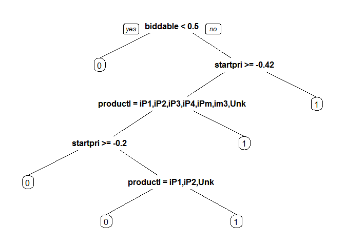
 predict_cart <- predict(model_cart1, newdata = test, type = "prob")[,2] ROCRpred = prediction(predict_cart, test$sold) as.numeric(performance(ROCRpred, "auc")@y.values) ## [1] 0.8222028

このモデルは、以前のものよりも悪い評価をしています。 相互検証によってパラメーターを選択して、結果を改善してみましょう。モデルの複雑さを決定するcpパラメーターを選択します

 library(caret) ## Loading required package: lattice ## Loading required package: ggplot2 ## ## Attaching package: 'ggplot2' ## ## The following object is masked from 'package:NLP': ## ## annotate library(e1071) tr.control = trainControl(method = "cv", number = 10) cpGrid = expand.grid( .cp = seq(0.0001,0.01,0.001)) train(sold ~ ., data = train, method = "rpart", trControl = tr.control, tuneGrid = cpGrid ) ## CART ## ## 1303 samples ## 29 predictor ## 2 classes: '0', '1' ## ## No pre-processing ## Resampling: Cross-Validated (10 fold) ## ## Summary of sample sizes: 1173, 1172, 1172, 1173, 1173, 1173, ... ## ## Resampling results across tuning parameters: ## ## cp Accuracy Kappa Accuracy SD Kappa SD ## 0.0001 0.7674163 0.5293876 0.02132149 0.04497423 ## 0.0011 0.7743335 0.5430455 0.01594698 0.03388680 ## 0.0021 0.7896359 0.5714294 0.03938328 0.08143665 ## 0.0031 0.7957780 0.5831451 0.04394428 0.09055433 ## 0.0041 0.7919612 0.5748735 0.03867687 0.07958997 ## 0.0051 0.7934997 0.5775611 0.03727279 0.07705049 ## 0.0061 0.7888843 0.5678360 0.03868024 0.08040614 ## 0.0071 0.7881210 0.5662543 0.03710725 0.07714919 ## 0.0081 0.7888902 0.5678010 0.03657083 0.07592070 ## 0.0091 0.7888902 0.5678010 0.03657083 0.07592070 ## ## Accuracy was used to select the optimal model using the largest value. ## The final value used for the model was cp = 0.0031.

提案された値を挿入し、結果のモデルを評価します

 bestcp <- train(sold ~ ., data = train, method = "rpart", trControl = tr.control, tuneGrid = cpGrid )$bestTune model_cart2 <- rpart(sold ~ ., data = train, method = "class", cp = bestcp) predict_cart <- predict(model_cart2, newdata = test, type = "prob")[,2] ROCRpred = prediction(predict_cart, test$sold) as.numeric(performance(ROCRpred, "auc")@y.values) ## [1] 0.8021447

ランダムフォレスト

理論上最も複雑なモデルの結果を見てみましょうが、非常に簡単に使用できます- ランダムフォレスト

 library(randomForest) ## randomForest 4.6-10 ## Type rfNews() to see new features/changes/bug fixes. ## ## Attaching package: 'randomForest' ## ## The following object is masked from 'package:dplyr': ## ## combine set.seed(1000) model_rf <- randomForest(sold ~ ., data = train, importance = T) predict_rf <- predict(model_rf, newdata = test, type = "prob")[,2] ROCRpred = prediction(predict_rf, test$sold) as.numeric(performance(ROCRpred, "auc")@y.values) ## [1] 0.8576486

ご覧のように、モデルはすでに使用されているすべての中で最良の結果を示しています。不要な変数を排除することで改善を試みましょう。これは、変数の重要性を評価するための組み込みモデルを持つのに役立ちます。

 varImpPlot(model_rf)

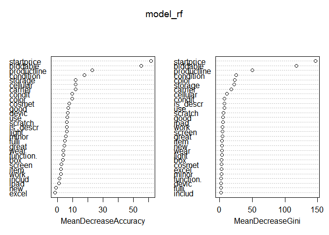
左のグラフでは、モデルの品質を改善しない兆候があることがわかります。それを削除し、結果のモデルを評価します。

 set.seed(1000) model_rf2 <- randomForest(sold ~ .-excel, data = train, importance = T) predict_rf <- predict(model_rf2, newdata = test, type = "prob")[,2] ROCRpred = prediction(predict_rf, test$sold) as.numeric(performance(ROCRpred, "auc")@y.values) ## [1] 0.8566796

評価では、モデルは改善されなかったことが示されましたが、常識に基づいて、製品の説明にexcelという単語が存在しても販売に影響する可能性は低く、モデルの簡素化（品質に大きな損害を与えることなく）は解釈を改善します。

したがって、調査したすべてのモデルの最良の結果は、ロジスティック回帰を示しました。その結果、公開委員会（利用可能なすべてのテストデータの50％の見積もり）では、結果が0.84724のモデルは1884年から211を取得しましたが、最終プロトコルでは1291に低下しました。

次回は、 Digit Recognizerタスクの例を使用して、トレーニングサンプルのサイズがモデルの品質にどのように影響するか、同じタスクでの主成分法の適用について説明する予定です。その後、 Bag of Words Meets Bags of Popcornコンペティションに参加した経験と、有名なTitanic：Disasterからの機械学習タスクでの長い研究について話します。

最後に、データ分析コースに参加することをお勧めします。私の経験では：

有用で実用的な方法のみが記載されています。
重点は、単なるソリューションではなく、タスクで達成する必要がある結果にあります
本当にやる気を起こさせ、一生懸命働きます

じゃあね！

データサイエンスで1か月に大量にポンプを使用する方法