Introduction
Very often, as in the exact sciences (physics, chemistry), and in other areas (economics, sociology, marketing, etc.) when working with various kinds of experimentally obtained dependences of one quantity (Y) on another (X), there is a need to describe the received data by some mathematical function. This process is often called expression , approximation , approximation, or fitting .
Most often, a linear function is used for data fitting:
Indeed, it is quite simple mathematically, it’s convenient to work with it, the meaning of the parameters A and B is crystal clear even to a middle school student, for it there are well-functioning mathematical methods that allow them to be unambiguously and quickly found, and most importantly, many experimentally obtained dependencies on in fact, they have a linear nature to one degree or another.
Lyrical digression
It will be important to mention the situation where the same experimental data can be described quite well (within the framework of predefined metrics) by very different mathematical functions, as shown in Fig. one.
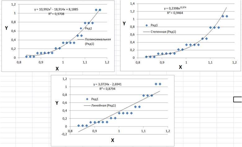
Fig. 1. An attempt to describe the same set of experimental data by quadratic, power, and linear functions.
An unambiguous report, but which is better, does not exist. Everything is determined by those tasks (to obtain the area under the curve, find out the value of the derivative, find out the new value of Y for another X, etc.), for the solution of which it is proposed to use one or another mathematical approximation. Of course, the most useful information can be obtained from the mathematical approximation, which not only perfectly describes the experimental data, but behind which is the physical / chemical / economic, etc. model of the dependence observed in the experiment. Then, useful information is extracted from the obtained optimized parameters.
There are situations when the experimentally obtained dependence is more complex and the use of linear approximation becomes meaningless and it is necessary to involve other mathematical functions, Fig. 2-A.
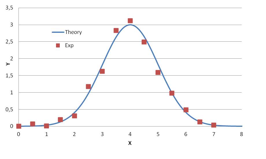
Fig. 2-A. An abstract example of a nonlinear experimental dependence of Y on X (red dots) and its theoretical approximation (blue curve) by the Gauss function.
For fitting non-linear experimental dependencies, there are a number of software solutions (Matlab, Origin, Datafit, etc.). It does not cause great difficulties to implement such a fitting in MS Excel (remember about solver).
However, there are situations when the experimental curve consists of several individual curves that are completely or partially superimposed on each other and independent by their nature. This is especially often manifested in physical and chemical measurements: infrared spectroscopy (Fig. 2-B), nuclear magnetic resonance (Fig. 2-C), X-ray photoelectron spectroscopy (Fig. 2-D), chromatography (Fig. 2-D) etc. In some cases, small but very proud an important peak is completely or almost completely hidden by a large peak, so that it is almost invisible to the naked eye. And its existence has to be guessed for indirect reasons.
| Examples |
|---|

Fig. 2-B. An example of overlapping peaks in the FTIR spectrum. On the Y axis (not shown) is a dimensionless quantity characterizing the absorption of IR radiation by a substance, along the X axis is the wave number in cm -1 . Source: Canadian Journal of Microbiology 63 (12), October 2017 . |

Fig. 2-c. An example of overlapping H1-NMR peaks. A source. |
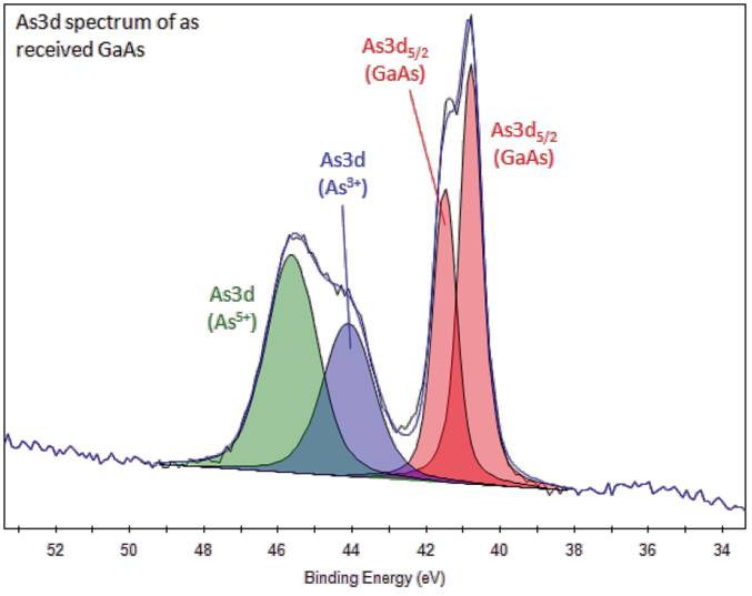
Fig. 2-g. Peak overlap in the As3d-XPS spectrum of a gallium arsenide (GaAs) sample. Various electronic states of As in the sample are clearly visible. The quantitative analysis performed using the fitting allows researchers to analyze the structure of the sample. Source |
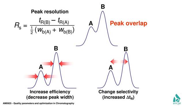
Fig. 2-D Examples of overlapping chromatographic peaks. The concentration of the analyte is directly proportional to the area under the peak curve, so you need to be able to accurately determine this area . Source |
Depending on the field of science, where similar situations with peak overlap occur, researchers have learned how to solve them differently. In NMR, the magnetic field is increased, the temperature is lowered during the measurement, which leads to the separation (resolution) of the peaks. In other words, they use a hardware and methodological solution to the problem, which is no doubt good in the context of improving instruments and methods, but often costs a lot of money and is not always available.
In infrared spectroscopy, they don’t do much with poorly separated peaks, they cannot be separated by hardware, and historically everyone is used to the fact that a peak is represented in the spectrum, for example, as a shoulder against the background of another peak and quite rarely, someone tries to extract more complete information from such a spectrum by fitting it (J. Braz. Chem. Soc., Vol. 19, No. 8, 1582-1594, 2008).
At the same time, in x-ray photoelectron spectroscopy, it is almost always necessary to fit experimental data as a superposition of several individual peaks (in the form of a Gaussian curve), which is realized by means of special software,
supplied with the device.
To separate the peaks in liquid and gas chromatography, the concentrations of substances are reduced, additional separation columns are installed, their lengths are increased, chemical modification methods are used, the conditions for chromatographic separation are changed, etc. But, oddly enough, despite the urgency of the problem, use the mathematical capabilities of peak separation. Although there are appropriate methods and models , they have not yet found their application in commercial chromatographic solutions ...
Despite the need to carry out multi-component (multi-functional) fitting, the author of these terms is not familiar with software that allows using several identical or different mathematical functions for fitting simultaneously. In the wonderful program OriginPro 8, multifitting is limited by the functions of Lorentz and Gauss, which is not bad, but not enough. At the same time, the quality of the fitting is not always satisfactory and there is no way to control the fitting process itself. If you did not like its results, then you have to start the process from the very beginning and so many times ....
Another not unimportant moment is the fact that almost all programs, when performing fitting, work only with this signal Y and do not automatically perform a derivative of this signal fitting, which can lead to insignificant results.
Therefore, when the real problem arose to describe the experimental curves, from the shape of which it was clear that multifunctional fittings could not be dispensed with, a suitable tool was not at hand. And I also wanted the visibility and controllability of the fitting process and that the experimental and calculated derivatives coincide. Of course, the problem could be solved manually in MS Excel, but there was a lot of data and I wanted to practice it in Python, which a few months earlier I began to study as my first programming language.
In this context, the following goal was set.
purpose
Write a program for convenient, intuitive, fast and high-quality multifitting of loaded experimental data, taking into account the fitting of the signal itself and its derivative.
In this case, the user must manually set the number of various mathematical functions used in the fitting and be able to select one or another mathematical function from the list.
In the process of fitting itself, I wanted to be able to control the process of selecting parameters myself, and not to trust optimization algorithms in the blind, primarily because they do not take into account the coincidence of the derivatives of the experimental and calculated signals.
Plus other little things, such as smoothing out noise and removing "artifacts" from the original data that interferes with the calculation of the derivative.
results
Given the lack of experience in programming, the task seemed not simple, but very interesting, which we had to solve, breaking it into subtasks:
- Reading / writing data;
- Converting the inconvenient format "07/17/2019 14:55:38" of the date and time values to relative minutes convenient for work;
- Studying the basics of Matplotlib for outputting data in the form of graphs and dynamically changing function parameters through the built-in gadget. The corresponding corresponding site helped a lot ;
- The use of a simple (5-point) method of smoothing and replacing duplicates encountered in the data array (along the X axis) with the corresponding linear approximation;
- Numerical integration and differentiation of data;
- Creating a graphical interface and learning the basics of OOP for this.
There probably isn’t much point in describing the details, questions and problems that arose during the writing of the program. Details are available to the code itself, the code is available here . Most of the questions and problems turned out to be standard, the full or partial solution of which was on various sites and in books devoted to Python, as well as on stackoverflow . Solutions and Examples stupidly copied sorted out and adapted to your needs. Below is a brief description of the program, its capabilities and limitations at the moment. The program consists of three working files and a brief instruction:
Fitting_tool.py -Interface, checking the correctness of parameter input, calling various functions.
NumPy1.py - A class of methods for reading, writing, processing data and displaying them graphically
ThFunction.py - A class of several mathematical functions, their parameters with initial values and the boundaries of the intervals of variation of these parameters.
Fitting Tool v.1.0 Help.pdf - A small manual with pictures, which I decided to do immediately in English.
When starting the program, it is proposed to open a file with your data or use the existing examples that you need to import.
Then you can view the original graph and its derivative, calculated as it is or after mathematical smoothing. It is not easy to say in advance which smoothing method will work better and it makes sense to try them all or choose the option without smoothing. As a result, a standard window appears with a graph of the experimental signal and its derivative, Fig. 3-A.
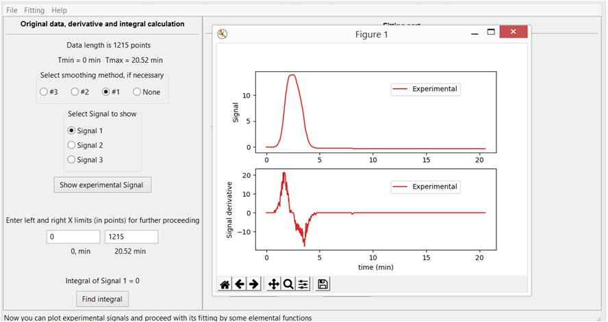
Fig. 3-A. A graphical representation of the original experimental signal and its derivative using one of three methods of mathematical smoothing.
Having set the left and right boundaries of the considered interval, we can focus the graph and subsequent calculations on the area of interest, Fig. 3-B.
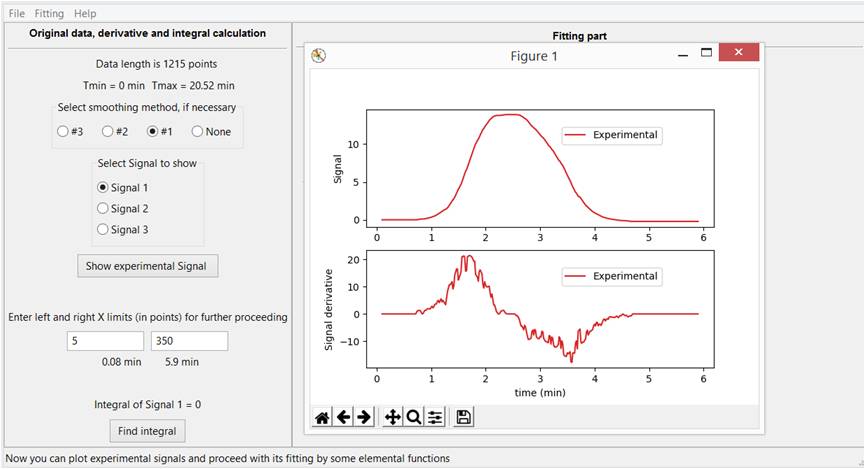
Fig. 3-B. Defining the left and right boundary of the interval of the most interesting part of the experimental curve for further fitting.
On the right side of the program, you can set the number of mathematical functions used for fitting and select the type of each function used. Then it will be possible to set three values for each parameter of the selected function. Min, Max values correspond to the left (Min) and right (Max) boundaries of the numerical interval in which the user will search for the optimal parameter value. The value Def (Min <Def <Max) shows the initial, it is the current value of this parameter, Fig. 4.
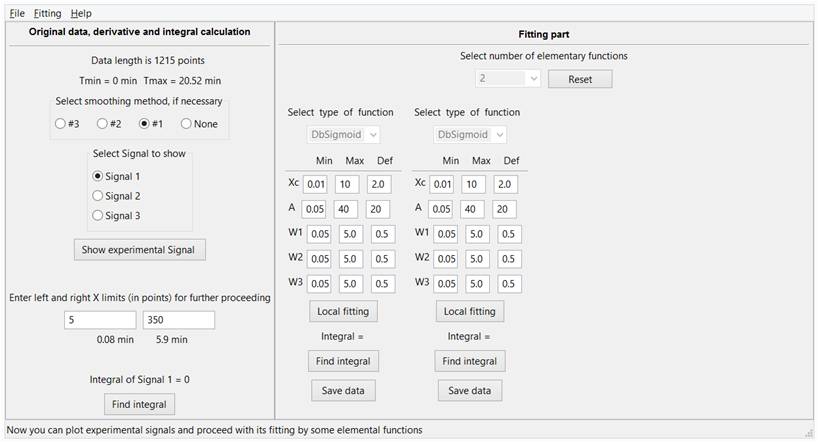
Fig. 4. The choice of the number and type of mathematical functions that will be used in the fitting. If necessary, the user can change the values of Min, Max and Def for each of the parameters of each function.
Further, either, remaining within the framework of one selected function, the user can perform the fitting (Local fitting) of its parameters, or through the Fitting \ Global fitting menu, optimize the parameters of the global function, which is a superposition of two (or more) local functions.
To begin with, it is convenient to “zero” the amplitude of the second function and achieve some (not necessarily perfect) coincidence of the profiles of the left (or right) part of the experimental signal and its derivative with the corresponding part of the first function and its derivative, Fig. 5-A.
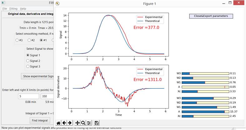
Fig. 5-A. Fitting with one function. Trying to get the best fit for the left side of the experimental curve. The amplitude of the second function is specially reduced to almost zero.
After receiving a satisfactory result, “turn on the second function” in the game (Fig. 5-B) and find the optimal parameters for it. In the process of fitting it, you can return to the parameters of the 1st function and make sure that the error is at a global minimum in all its parameters.
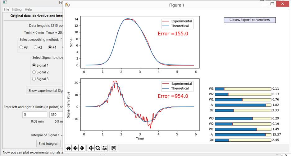
Fig. 5 B. A fitting with two functions gives a better description of the original signal and its derivative (ignoring the remaining noise in the derivative graph).
The "Close & Export parameters" button allows you to close the window with the graph and export the current parameters to the main program window, where you can set more convenient Min and Max values for the selected parameters and continue to reduce the error again through Fitting \ Global fitting.
Error - it’s the metric of approximation quality of the original signal and its derivative is determined by the standard formula:
where SE i and ST i are the experimental and calculated signal values. N is the number of points in the array, and a factor of 1000 is chosen for convenience. A similar formula is used to assess the accuracy of the fitting of the derivative of the signal, however, due to the presence of possible noise, it cannot be completely "zeroed", and this is not necessary, because matching curve profiles is enough.
If two functions are not enough for a high-quality fitting, then you can reset the settings with the Reset button and select a larger number of functions.
At the moment, the program contains six mathematical functions:
| Reduction | Title | Formula and Options | Graph example |
| --------------- | ------------ | -------------------- -------- | ------------------ |
| DbSigmoind | Double sigmoid |
Parameters: A, Xc, W1, W2 and W3 | ! [image] (https://habrastorage.org/webt/8t/bk/qf/8tbkqfwko9dxi7twikbsnuejxiq.jpeg) |
| Sinus | Sinus |
Parameters: A, w and phi |! [Image] (https://habrastorage.org/webt/aw/9q/of/aw9qofy0dqcgmlu7n55l64alin4.jpeg) |
| Gauss | Gauss function |
Parameters: A, b and c |! [Image] (https://habrastorage.org/webt/ll/t8/bd/llt8bditpjizexuqjt7hweefore.jpeg) |
| Exp | Exponential Function |
Parameters: A and b |! [Image] (https://habrastorage.org/webt/ru/43/yf/ru43yf0ixgrukkb2okfhkghhtfe.jpeg) |
| Lorenz | Lorentz function |
Parameters: A, x 0 |! [Image] (https://habrastorage.org/webt/ko/e8/d-/koe8d-v0nxvng0mc0omyjz2jyco.jpeg) |
| Sigmoid | Sigmoid |
Parameters: A, B and C |! [Image] (https://habrastorage.org/webt/d0/ls/cr/d0lscrate33shcqmb227djxs8au.jpeg)
|
It was decided to rest on our laurels and limit version 1.0 to these six mathematical functions. Those who wish can easily add a new mathematical function to the ThFunction.py file and add the condition for determining its parameters to the “F_Option” function of the Fitting_tool.py file according to ready-made templates from comments in files.
In future versions, if there is interest in this topic, I will try to add the ability to the user to enter their mathematical functions in the program itself.
###Conclusions
A convenient tool was created that allows manual multifitting of experimental data, while simultaneously controlling not only the shape and error of the calculated signal, but also the shape and error of its derivative.
Work on the project brought great pleasure and allowed to get the first practical programming experience.
I would like to hope that the created tool - Fitting tool will be really useful to someone else.