The Life of John Conway
We believe that all programmers are well aware of the cellular automaton life (or evolution), invented by the English mathematician John Conway in 1970. Perhaps some even pored over a self-written program simulating Conway's cellular automaton.
We briefly recall the essence of the model of Conway.
1. The model is a field finite or infinite (that is, closed) field consisting of cells.
2. Each cell can be either filled (that is, live) or empty (that is, dead).
3. The state of the field changes step by step, each subsequent state is calculated from the previous one according to the rules.
3.1. In a dead cell, next to which there are exactly three living ones, life is born.
3.2. If there are two or three living cells next to a living cell, then it continues to live.
3.3. If there are less than two or more than three living cells next to a living cell, then it dies (that is, either from loneliness or from overpopulation).
Despite the simplicity of the rules, the model impresses with its similarity to the development of populations of primitive organisms. Probably, everyone was visited by the idea that, by slightly modifying the rules, it is possible to achieve even greater similarity of the model with the behavior of living organisms.
New life
The new model will also be an infinite (closed) field consisting of cells. In each cell, only one simple organism can be located, which we will arbitrarily call a plant. Initially, the field may contain in each cell a certain amount of the resource necessary for plant nutrition.
We will give the plant the following parameters: a) initial mass (in units), b) nutrition (in units), c) life expectancy (in measures), d) reproductive age (in measures), e) number of seeds for reproduction.
The field status will also change step by step according to certain rules.
1. With each step, the mass of the plant increases by the amount of nutrition b . Accordingly, the mass of the resource in the cell where the plant grows decreases by the same amount. If the cell no longer has a resource for nutrition, the plant dies of hunger.
2. The age of the plant increases with each measure by one.
3. Having reached reproductive age d , or maturity, the plant scatters seeds in the neighboring cells (the so-called Moore neighborhood) of quantity e , each of which has an initial mass of a . In this case, the mass of the parent plant decreases by the total weight of the seeds. Seeds may be less, since the mass of the parent plant cannot be less than the initial mass a . If a seed enters a cell that is already occupied, then it turns into a resource.
4. Having reached the maximum age c , or life expectancy, the plant dies of old age. The mass of the deceased plant increases the mass of the resource in the cell.
The following conclusions immediately follow from these rules.
Conclusion 1. The total mass of resources and plants at any time in the system is constant.
Conclusion 2. If there is less resource in the cell than the plant needs to reach maturity (that is, the bd value), then the plant will die without giving offspring.
Experiment 1.1. Favorable environment
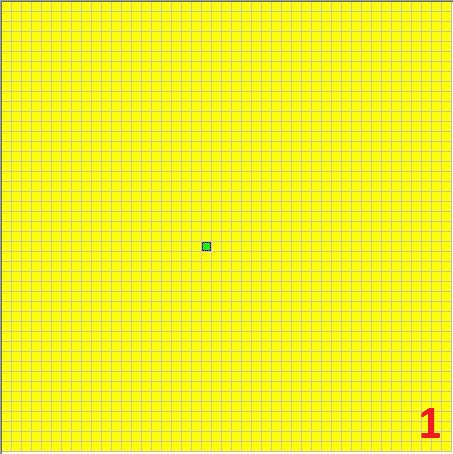
We put in the field one plant of the Lime species, from which we determine the values of the parameters: a) initial mass - 1 unit, b) food supply - 1 unit, c) life expectancy - 10 measures, d) reproductive age - 5 measures, e) number of seeds for reproduction - 3 pieces.
From these values we conclude that the cell of the field must contain at least 5 units of the resource for the growth and reproduction of the plant. Evenly fill the field so that each cell contains 7 units of the Yellow resource (Fig. 1), and start the modeling process. The Lime species will quickly breed and fill the entire habitat (Fig. 2).

Conclusion 3. Under favorable conditions, the species quickly covers the entire available habitat.
Conclusion 4. Under favorable conditions, life can continue almost indefinitely.
Experiment 1.2. Adverse environment
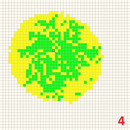
We place the same species of Lime plant (experiment 1) in another field, where the amount of resources is limited, and, accordingly, the habitat is limited (Fig. 3). Having started the modeling process, we can observe how the species, despite the restriction, slowly increases its habitat (Fig. 4).

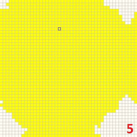
The range increases, however, in each individual cell, the amount of the resource decreases. Finally, the cells cease to have enough resources to reach maturity, and the species dies out (Fig. 5).
Conclusion 5. The species seeks to increase its habitat.
Conclusion 6. In the process of life, resources are distributed throughout the field almost uniformly.
The species failed to survive in an unfavorable environment, as it turned out to be unfit. If in this experiment the values of some parameters are changed for the Lime species, then survival can be achieved. For example, you can reduce the reproductive age of a plant to 3 measures.
However, manually selecting values is not so exciting. But let's not get ahead of ourselves and continue.
Experiment 1.3. Competition
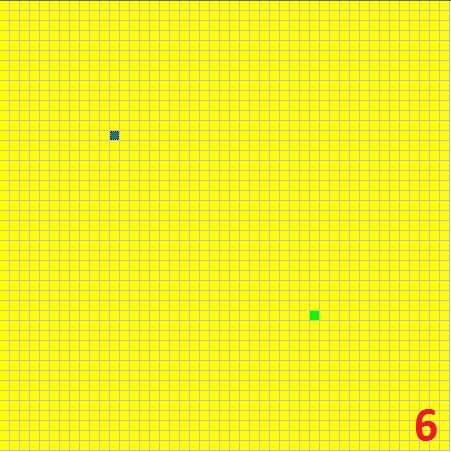
In the next experiment, in a favorable environment (a field uniformly filled with the Yellow resource) we place two types of plants - Lime and Teal (Fig. 6). The values of the parameters for both species are the same (experiment 1), they differ only in color so that they can be distinguished visually.
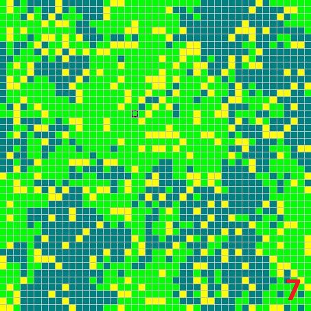
Having started the modeling process, we can observe how plants fill the entire field (Fig. 7). Of course, these two species cannot obviously fight each other, but they coexist on the same field, competing with each other. Sometimes one species reproduces more, sometimes another species, although none of them has an advantage over the other.
It is possible that this confrontation does not last forever, and one of the species, having bred, survives the other. But life in a favorable environment will continue anyway.
Conclusion 7. If species are equally adapted to the environment, then it cannot be said with certainty which of them will survive and which will die out.
Experiment 1.4. Symbiosis
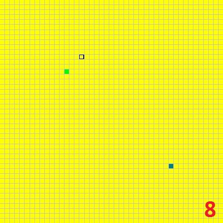
We evenly distribute two resources across the field: Yellow and Olive. We place in the favorable environment the same two types of plants Lime and Teal (Fig. 8). All parameter values are identical and the same as in the first experiment, but with a small exception. The Lime species feeds on the Yellow resource, and after death turns into the Olive resource. The Teal species feeds on the Olive resource, and after death turns into the Yellow resource. The relationship between the two plant species is obvious: they can only survive together.
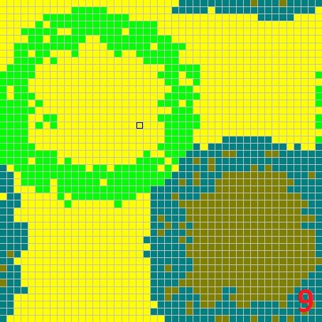
Having started the modeling process, you can see how at first the species diverge in circles from the original cell (Fig. 9), each eating its own nutritional resource in the cells. Then, as expected, the species change their habitat (Fig. 10). Unlike the previous experiment, by over-breeding one species creates better conditions not for itself, but for its counterpart.
Conclusion 8. With the interdependence of the two species, the extinction of one species will immediately entail the extinction of the other.

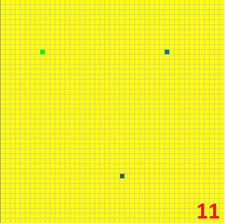
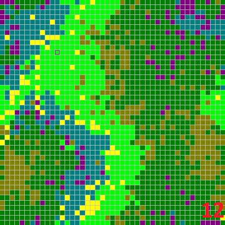
Let's complicate the experiment. Fill the field with three resources of Yellow, Olive, Purple and place in the resulting environment three interdependent species of plants - Lime, Teal and Green (Fig. 11). All parameter values are identical and the same as in the first experiment, but with a small exception.
The Lime species feeds on the Yellow resource, and after death turns into the Olive resource. The species Teal feeds on the Olive resource, and after death turns into the Purple resource. The Green species feeds on the Purple resource, and after death turns into the Yellow resource.
Having started the modeling process, over time one can observe curious wave-like (Fig. 12) or spiral-shaped (Fig. 13) structures consisting of different species. The extinction of one species will immediately entail the extinction of the two remaining species.

Conclusion
Despite the simplicity of their appearance, cellular automata present quite wide possibilities for modeling various systems, and in a short article we tried to present some interesting examples of modeling simple pseudobiological systems.
Perhaps the conclusions made in the article are pretty obvious, but in this case they are all backed up by simulation results.
Sources
en.wikipedia.org/wiki/Life_Game
en.wikipedia.org/wiki/ Cellular Automation