Start of Review
So, my dear colleagues, we begin the review with what we really want to highlight here. In the article I want to consider the elements that are typical for building an industrial controller program, and show how they can be applied to home automation systems. And the most important thing is to find the answer to the question - what is needed for this.
Home Automation - Applications
Home, sweet home ... Do you really need a controller? The answer is simple - it all depends on what is available in such a house. Of course, if you just have an apartment, and the automation consists in managing your home media center and air conditioning in the summer, everything that is written below can be completely uninteresting. But if your hobby is not only pushing the couch (what is there to hide, I myself have sometimes noticed this), then the article can be very useful.
So, let's try to understand how improvised means can simplify our difficult life. As an example, we use the real situation - one pump in a well 70 meters deep, which two neighbors put into a fold. They installed it in the spring, when there was a lot of water in the well, and in general, it was just warm and good. But time passes, and questions begin - to raise water from such a depth, you need electricity, for which you have to pay. The basement and the technical floor were flooded several times - they simply forgot to turn off the pump ... Yes, and it’s not very convenient to manually control it — you need to close one tap, open another, then turn on the pump and watch the water level in the tank.
Is it worth it to spend your time on it, which is already lacking? An inquiring mind begins to search for solutions, and of course, finds it! A list of tasks for implementation is born.
- Payment for consumed electricity does not have to be common - that means, we will install two starters, each of which is connected to its own electric meter.
- The pump should not fail due to lack of water - which means we will install a sensor for the pump’s “dry” stroke. If there is no water, we simply do not start the pump, and if it works, we emergency stop.
- The pump should not run for too long - for example, more than 25 minutes. Exceeding this time indicates that the system is leaving its normal mode of operation.
- Filling the containers should take place without human intervention, that is, automatically. And this means starting at the lower level and stopping at the upper level.
- Only one tank should be filled, that is, we install two valves - to supply water for a set in each tank.
- The pause between pump starts must be at least 30 minutes.
- A power interruption should not affect the operation algorithm, if it was active. Despite everything, the algorithm must be completed.
The tasks are simple, and they can be solved in a hundred, if not a thousand ways. But the title of the article speaks for itself, and we will go on a thorny path. Let's use a virtual (for now, of course) controller, which will do all this.
How does an industrial controller work?
Of course, we’ll immediately clarify - we are talking about the so-called programmable logic controllers, or PLC for short. What is hiding under this abbreviation? And here is what is hidden - an incredible variety of hardware solutions, a huge number of software products and utilities. A reasonable question immediately arises - how then to use all this good? Is it really necessary to study the material part from scratch and find time and money for each new device in order to take training courses and gain the skills necessary to work with each device?
The answer is no, it is not necessary. Everything is already done before us. It remains only to study and learn how to use. This is what I propose to do next - to dive a little into the IEC 61131 standard. Let's reveal what parts this standard contains.
- IEC 61131-1: General information.
- IEC 61131-2: Equipment requirements and testing.
- IEC 61131-3: Programming Languages.
- IEC 61131-4: User Guide.
- IEC 61131-5: Communications.
- IEC 61131-6: Functional safety.
- IEC 61131-7: Fuzzy control programming.
- IEC 61131-8: Guidelines for the use and implementation of programming languages.
- IEC 61131-9: Single-point digital communication interface for small sensors and actuators.
- IEC 61131-10: PLC open XML based interchange format.
But we won’t delve into the topic of standards, and simply put, the controller generally works cyclically - polling the status of inputs, the interpreter executing the control program, setting the status of the outputs, performing internal maintenance tasks and again returning to polling the status of the inputs. Boring enough, but effective and efficient. A control program is a pseudo-code that is created using a programming environment. Usually, such a pseudo-code is a binary-coded sequence, which has nothing to do with the usual programming languages. Although for the user it is presented in a form that is understandable - for the controller, a completely different view is used. A good example is a small program, presented in the form of IL, LD and in the form of binary encoding for the controller (hmm, there is not even a special term). Below is a small example below the spoiler.
Program display options 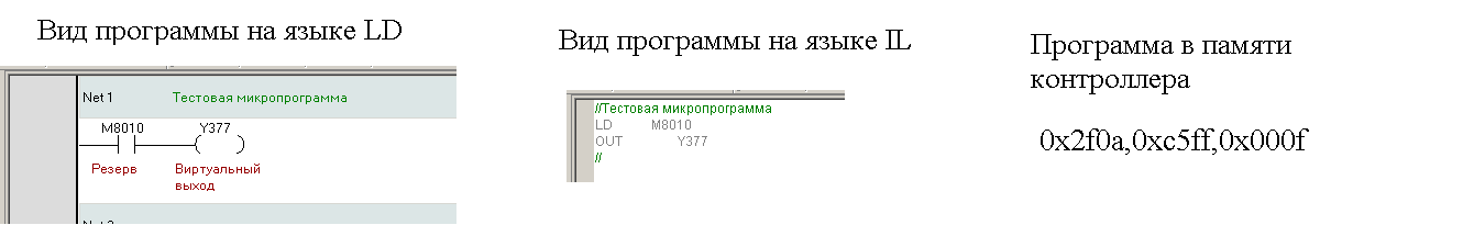
So what makes this program useful? Yes, she does nothing - if the value of M8010 is 1, then 1. will be written to the output with address Y377. Accordingly, the same is for 0.
One of the biggest advantages of this implementation is the ability to unload the program from the controller’s memory, open it for editing in an editor in a way that is understandable to humans, compile (this term is conditional here) and load it back into the controller’s memory. Moreover, some controllers even save comments and variable names.
How to program the controller?
Of course, specialized software is needed. After lengthy searches and experiments, Autoshop v3.02 from Inovance Control was chosen. It is remarkable in that it is free, available for free download, and it supports controllers that are compatible with Mitsubishi controllers. And it supports work not only through serial ports, but also through Ethernet. Link to the version used by us, under the spoiler.
Link to download from Yandex Disk
Well, we installed the program and now another question - how to write the program to our controller? Since we will work with a specific device, we will install specific virtual COM port drivers. To save conclusions, and to simplify, I decided to use the board's USB port for connection. Drivers under the spoiler.
Drivers on Yandex Disk
After installing the drivers and connecting the board via mini-USB, you can check if everything is successful with you. To do this, right-click My Computer-Management-Device Manager-Ports (COM and LPT). You should see such a window as under a spoiler. The COM port number on your system may vary.
device Manager 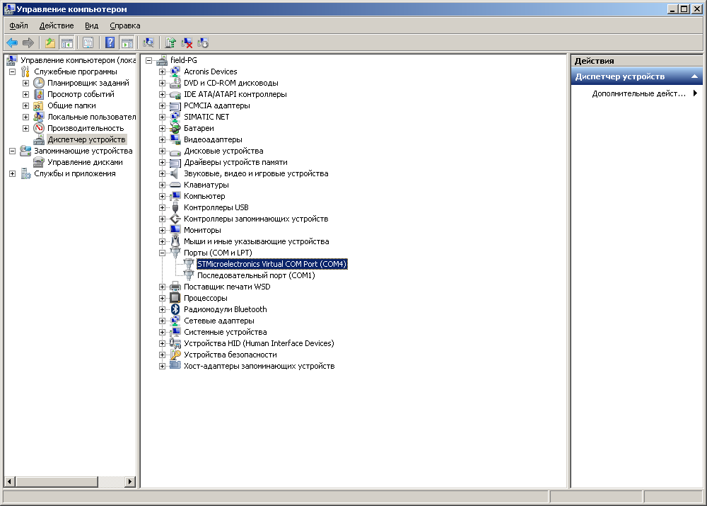
Now you can select Tools-Communication Setting in the AutoShop program menu, select Serial in the window that appears, specify the port number and click the Test button. You should have such a window like under a spoiler.
Successful connection to the board 
But if something doesn’t work out for you, write either in PM or in a comment. We will definitely help.
Elements of the program, without which it will be sad
Hereinafter, we will consider the language of ladder diagrams, or the so-called LD. Let us consider only those elements that we will use later.
- The inputs and outputs are discrete. They are designated as X and Y. Designed for receiving and issuing discrete signals.
- The memory area of M merkers M. It can take two states - on and off.
- Timers are designated T. Designed for counting time from 0.1 to 3276.7 seconds.
- The area of registers D. It has a cell dimension of 16 bits, but can also be addressed as a 32 bit cell.
Spherical horse in a vacuum, or indirect addressing registers
The indirect address registers are designated V and Z and can be addressed from V0 to V7 and from Z0 to Z7. Why can they be used? Let's look at how they generally work. This crazy-looking D1000V0 record means that the cell address calculated as D1000 address plus the value written to the indirect addressing register will be used. If there is 15, then we will use the address of cell D1015. It is very convenient when working with data arrays or with table control - it is enough for us to change the value of the index register, and we get the values from those memory cells that were addressed. But while we will not apply them, we will touch on this in the next publication.
A little bit about the visualization of the program, or online debugging
If you are a programmer and have just finished writing a program, the next step is debugging. And here the question arises - how to do it. Again, there are a lot of options, but I will talk about the one that we will use further. The programming environment editor allows you to visually show what values of bits and variables are currently in the controller memory by pressing one button. A very revealing example will be - below the spoilers offline and online display of the program in the editor.
Button for switching to the variable view mode 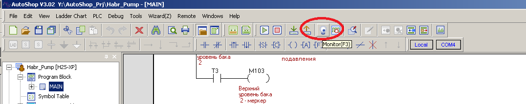
View of the program in the mode of viewing the values of variables 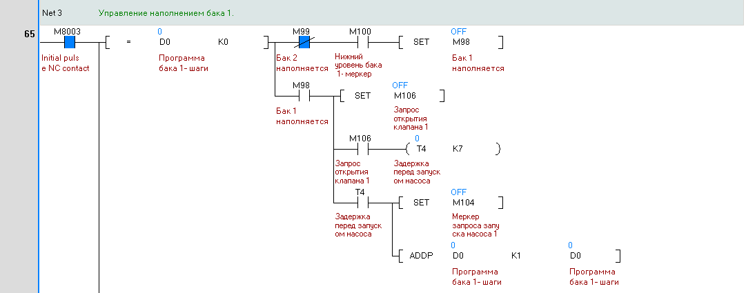
Type of program in edit mode 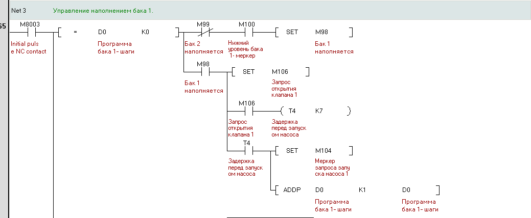
A little more about the processes that occur when you click the Online button. The program quickly compiles a list of visible variables, and upon completion, writes it to a specific controller buffer. After that, the controller prepares data from this list and places it in another buffer. The program reads the values from this buffer and displays them as values on the mimic diagram. If you scroll a little program in the display window and change the visible variables, this cycle will repeat again ...
Who calls Hamlet, or on stage BluePill x405
Have you noticed that the market doesn’t come across simple boards like a blue tablet, but equipped with processors like F405 and higher? I personally came across only with F401 stones, but this is a slightly different level ... I’m easy to climb, and for my experiments, without thinking twice, I made a payment in the good old P-CAD 2006 and ordered from the Chinese on one of the quick order sites. Of course, in color it is a green tablet, but in meaning I decided to leave the name BluePill, but indicating that it is already x405. The result under the spoilers is a photo of the BluePill x405 board.
View from above 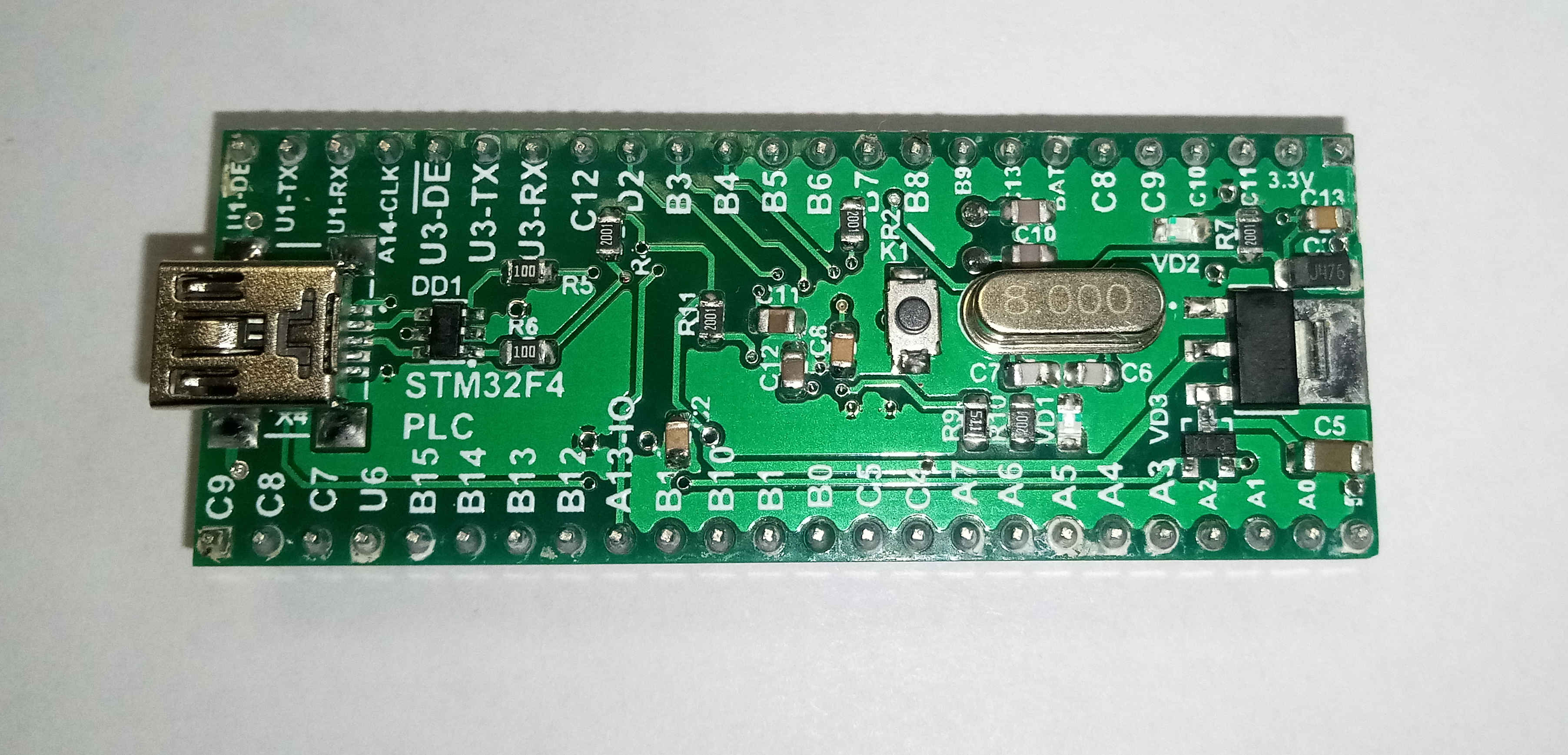
Bottom view 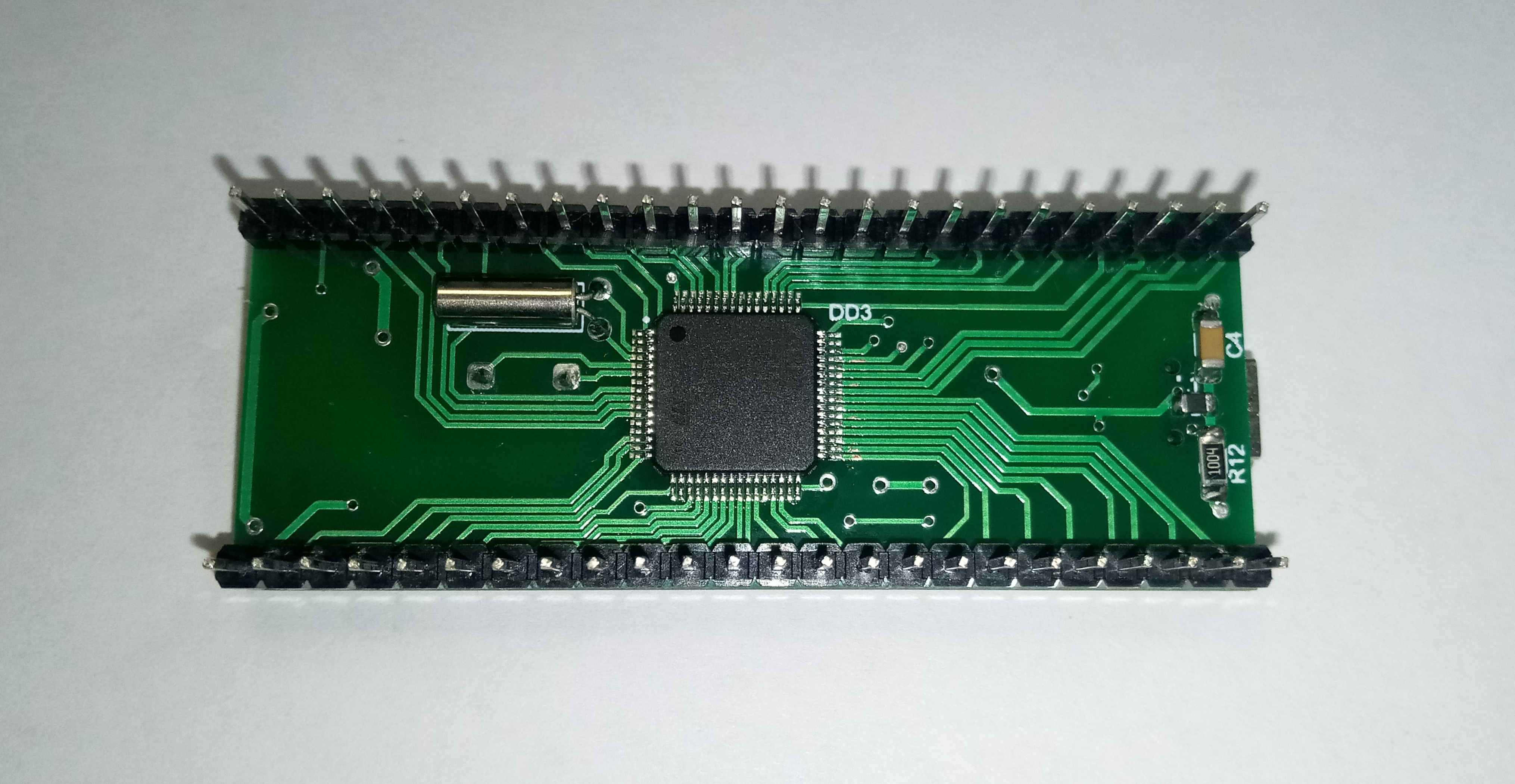
Concept and gerber on github
A little bit about why this board is so remarkable? After all, there were just thousands of attempts to create bluepill clones! But the difference is this: I attach firmware to this board, which will turn it into a kernel that runs a program that is compatible with the Mitsubishi industrial controllers in the command system. This miracle is calculated on 16 inputs, 16 outputs, 2 analog inputs, 3 UART with DE support for RS485, 1 onewire master bus. UART can work as a master bus modbus RTU, as well as a slave. And they can work completely independently.
But that is not all - if you connect a 3V battery to the VBAT pin, then not only the clock, but also the timers, counters, merkers and the first 1000 general-purpose registers D will be stored their values. And there are 8000 registers.
Anticipating questions, I will say right away - yes, the software is built on the basis of a real-time operating system. Yes, DMA is used wherever possible. These features allow working without significant changes in cycle time at high communication loads. This version is the second revision, revised and supplemented.
This board can be programmed as a GX FXDeveloper, and IEC Developer and GX Works.
The fate of the pump and two tanks
Let us now solve this problem - especially since all the tools for this are available. In order not to drag out much, I wrote a program, broke it into parts (the so-called networking, or work chains), and I will show each of them here and give comments.
Net 1 - first run of the program 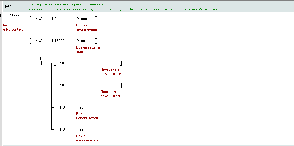
Register D1000 stores the time required to suppress contact bounce. In fact, the program already has this - but I want to show it more clearly. Register D1001 is responsible for the pump protection time. We write 15000, or 1500 seconds, in it. Next, we have a backup reset chain - if something goes wrong, you can send signal 1 to input X14 and restart the board. In this case, 0 is written to the registers D0 and D1, and the M98 and M99 merckers are reset.
Net 2 - input signal processing 
Here, with the help of timers, we get rid of the bounce of contacts. To do this, use a delay of 200 milliseconds. So that in the further program, when changing the contact's input address, it would not be necessary to rewrite a lot of chains, I use intermediate merkers (for example, M102). It is also noteworthy that the M8003 system merker is used here - it turns on after the first cycle of program execution has passed. But the M8002 Merker is active only in the first cycle of the program, and this can and should be used to set the initial values.
Net 3 - tank filling 1. 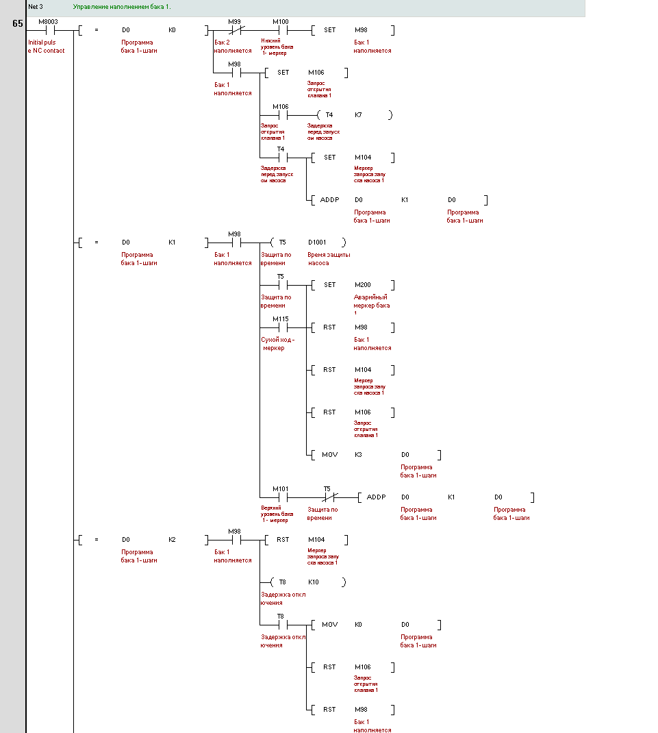
The filling of tank 1 is completely identical to the filling of tank 2 with the exception of the addresses. The drawing didn’t fit a bit - but you better look at it just by opening the project. What is remarkable about this control unit? The presence of protections and deadlocks that allow shockless start and stop mechanisms. For example, after opening valve 1, only after 700 ms a command will be issued to start the starter, which turns on the pump.
Management here does not provide for manual mode. Also, protection against dry running and protection against too long pump operation are implemented.
Net 5-6 - Output Management 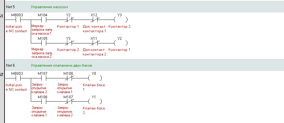
And here we control the outputs in compliance with the locks.
Of the tasks, only the connection of the 30 minute protection interval before restarting remained unfulfilled. I must say right away - in this version only the inputs X0-X3 and the output Y0-Y3 are implemented, which is quite enough for testing the material in this article. The binding is PA4-X0, PA5-X1, PA6-X2, PA7-X3 and PB4-Y0, PB5-Y1, PB6-Y2, PB7-Y3.
Program Cycle Speed - Grandfather Measurement Methods
When we ask ourselves this question, it immediately comes to mind to do so - to write to the controller a very large program from a certain number of identical elements, get the execution time and get the execution time of one command. It is said - done, under the spoiler program and in the name of the spoiler execution time.
7995 steps - 2.6 milliseconds
Here, each step is one command, and we get that 2.6 / 7995 = 0.325 microseconds. Not very fast, but not bad.
FPU - to be or not to be?
Now let's determine how quickly floating-point instructions work in our firmware. There are two firmwares, one using the built-in FPU, and the other with software emulation. The program below:
Program for calculating the execution time of an instruction
The firmware below is under the spoiler, and they have no restrictions
Two firmware
When using a hardware FPU, the program execution time is 1.8 ms, or 1.8 / 600 = 0.003 ms, or 3 microseconds.
Now replace the firmware - use software emulation. The result is already different - 2.5 ms, or 2.5 / 600 = 0.0041 ms, or 4.1 microseconds. Not bad, but the difference is quite noticeable.
Conclusion
Despite the large volume of the article, there are still a lot of materials that would be good to cover. So if this article is of interest to you, then this article will be followed by yet another. But I would like to find like-minded people who want to join the crossing of industrial and domestic with only one purpose - so that these tools are accessible to a simple layman.