A neural network for defining haters - “no, well it's a ban”

Hello!



Do you often see toxic comments on social networks? It probably depends on the content you are watching. I propose to experiment a little on this topic and teach the neural network to determine hater comments.



So, our global goal is to determine whether the comment is aggressive, that is, we are dealing with binary classification. We will write a simple neural network, train it on a dataset of comments from different social networks, and then make a simple analysis with visualization.



For work I will use Google Colab. This service allows you to run Jupyter Notebooks, and have access to the GPU (NVidia Tesla K80) for free, which will speed up learning. I will need the backend TensorFlow, the default version in Colab 1.15.0, so just upgrade to 2.0.0.



We import the module and update.

from __future__ import absolute_import, division, print_function, unicode_literals import tensorflow as tf !tf_upgrade_v2 -h
      
      

        
        
        
      

    
        
        
        
      
      

        
        
        
      

    
     

You can see the current version like this.

 print(tf.__version__)
      
      

        
        
        
      

    
        
        
        
      
      

        
        
        
      

    
     

Preparatory work is done, we import all the necessary modules.

 import os import numpy as np # For DataFrame object import pandas as pd # Neural Network from keras.models import Sequential from keras.layers import Dense, Dropout from keras.optimizers import RMSprop # Text Vectorizing from keras.preprocessing.text import Tokenizer # Train-test-split from sklearn.model_selection import train_test_split # History visualization %matplotlib inline import matplotlib.pyplot as plt # Normalize from sklearn.preprocessing import normalize
      
      

        
        
        
      

    
        
        
        
      
      

        
        
        
      

    
     

Description of used libraries

• os - for working with the file system

• numpy - for working with arrays

• pandas - a library for analyzing tabular data

• keras - to build a model

• keras.preprocessing.Text - for text processing, to submit it in numerical form for training a neural network

• sklearn.train_test_split - to separate test data from training

• matplotlib - to visualize the learning process

• sklearn.normalize - to normalize test and training data

Parsing data with Kaggle

I load data directly into the Colab laptop itself. Further, without any problems, I’m already extracting them.

 path = 'labeled.csv' df = pd.read_csv(path) df.head()
      
      

        
        
        
      

    
        
        
        
      
      

        
        
        
      

    
     

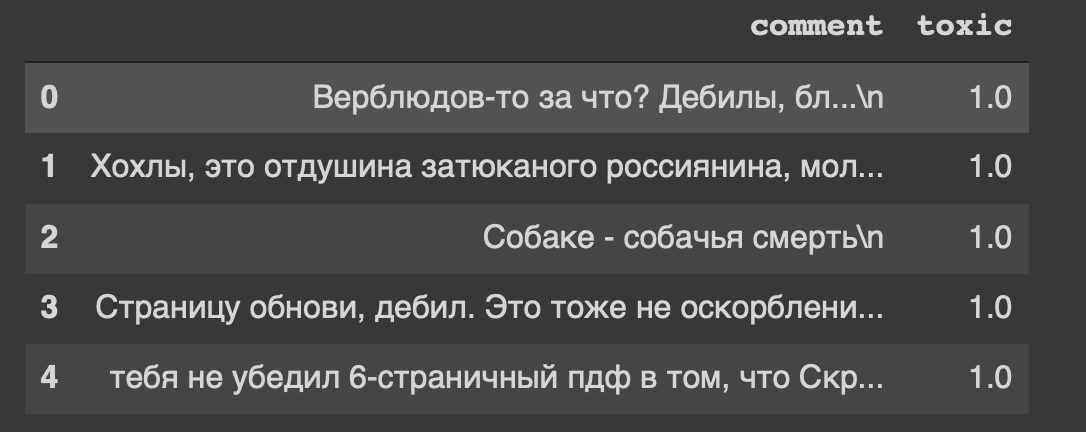
And this is the heading of our dataset ... I, too, somehow feel uneasy from "refresh page, moron."

So, our data is in the table, we will divide it into two parts: data for training and for the test model. But this is all text, something needs to be done.

Data processing

Remove the newline characters from the text.

 def delete_new_line_symbols(text): text = text.replace('\n', ' ') return text
      
      

        
        
        
      

    
        
        
        
      
      

        
        
        
      

    
     

 df['comment'] = df['comment'].apply(delete_new_line_symbols) df.head()
      
      

        
        
        
      

    
        
        
        
      
      

        
        
        
      

    
     

Comments have a real data type, we need to translate them into an integer. Next, save it in a separate variable.

 target = np.array(df['toxic'].astype('uint8')) target[:5]
      
      

        
        
        
      

    
        
        
        
      
      

        
        
        
      

    
     

Now we will slightly process the text using the Tokenizer class. Let's write a copy of it.

 tokenizer = Tokenizer(num_words=30000, filters='!"#$%&()*+,-./:;<=>?@[\\]^_`{|}~\t\n', lower=True, split=' ', char_level=False)
      
      

        
        
        
      

    
        
        
        
      
      

        
        
        
      

    
     

Quickly about the parameters

• num_words - number of recorded words (most common)

• filters - a sequence of characters to be deleted

• lower - a boolean parameter that controls whether the text will be lowercase

• split - the main symbol for splitting a sentence

• char_level - indicates whether a single character will be considered a word

And now we will process the text using the class.

 tokenizer.fit_on_texts(df['comment']) matrix = tokenizer.texts_to_matrix(df['comment'], mode='count') matrix.shape
      
      

        
        
        
      

    
        
        
        
      
      

        
        
        
      

    
     

We got 14k sample rows and 30k feature columns.







I am building a model from two layers: Dense and Dropout.

 def get_model(): model = Sequential() model.add(Dense(32, activation='relu')) model.add(Dropout(0.3)) model.add(Dense(16, activation='relu')) model.add(Dropout(0.3)) model.add(Dense(16, activation='relu')) model.add(Dense(1, activation='sigmoid')) model.compile(optimizer=RMSprop(lr=0.0001), loss='binary_crossentropy', metrics=['accuracy']) return model
      
      

        
        
        
      

    
        
        
        
      
      

        
        
        
      

    
     

We normalize the matrix and divide the data into two parts, as agreed (training and test).

 X = normalize(matrix) y = target X_train, X_test, y_train, y_test = train_test_split(X, y, test_size=0.2) X_train.shape, y_train.shape
      
      

        
        
        
      

    
        
        
        
      
      

        
        
        
      

    
     

Model training

 model = get_model() history = model.fit(X_train, y_train, epochs=150, batch_size=500, validation_data=(X_test, y_test)) history
      
      

        
        
        
      

    
        
        
        
      
      

        
        
        
      

    
     

I will show the learning process at the last iterations.

Visualization of the learning process

 history = history.history fig = plt.figure(figsize=(20, 10)) ax1 = fig.add_subplot(221) ax2 = fig.add_subplot(223) x = range(150) ax1.plot(x, history['acc'], 'b-', label='Accuracy') ax1.plot(x, history['val_acc'], 'r-', label='Validation accuracy') ax1.legend(loc='lower right') ax2.plot(x, history['loss'], 'b-', label='Losses') ax2.plot(x, history['val_loss'], 'r-', label='Validation losses') ax2.legend(loc='upper right')
      
      

        
        
        
      

    
        
        
        
      
      

        
        
        
      

    
     

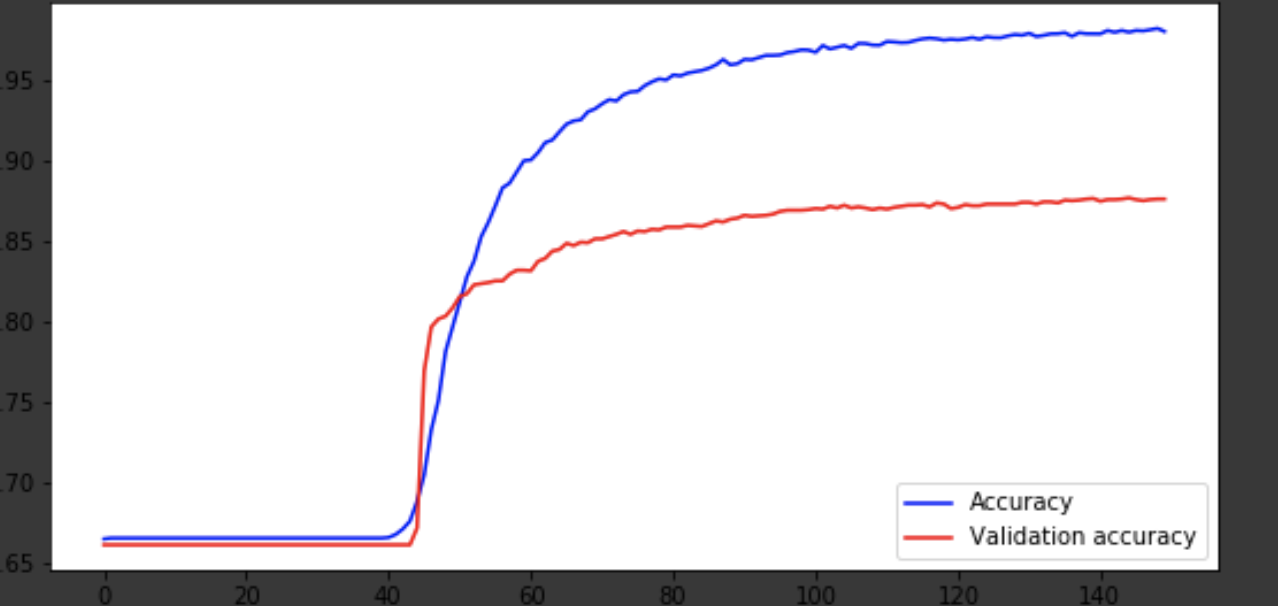
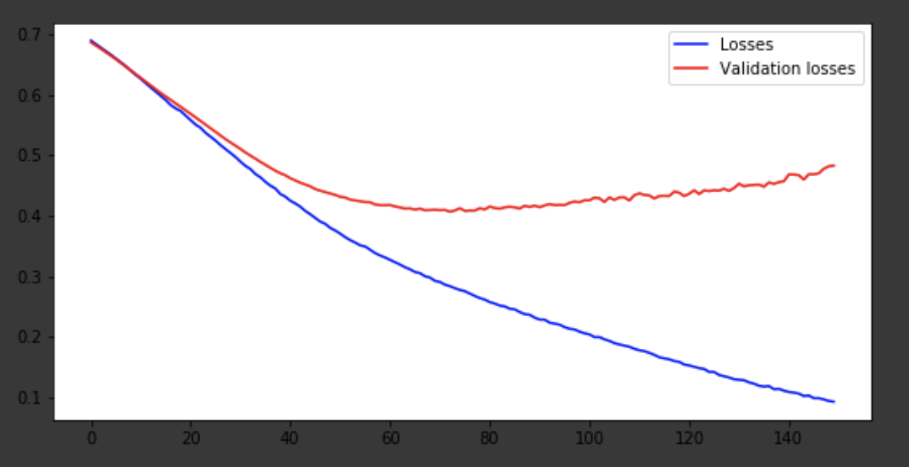
Conclusion

The model came out around the 75th era, and then it behaves badly. The accuracy of 0.85 does not upset. You can have fun with the number of layers, hyperparameters and try to improve the result. It is always interesting and is part of the job. Write about your thoughts in comments, let's see how many hats this article will gain.