
Every day the global web is replenished with articles on the most popular, most used machine learning algorithms for solving various problems. Moreover, the basis of these articles, slightly changed in form in one place or another, wanders from one data researcher to another. Moreover, all these works are united by one generally accepted, indisputable postulate: the application of one or another machine learning algorithm depends on the size and nature of the data available and the task at hand.
In addition to this, especially insisted data researchers, sharing their experience, emphasize: “The choice of an assessment method should partially depend on your data and on what, in your opinion, the model should be good” (“Data Science: insider information for beginners. Including R language, by Cathy O'Neill, Rachel Shutt) .
In other words, the statistics / data researcher should have not only experience in the subject field, but also a wide range of varied knowledge: “A data researcher is one who has knowledge in the following areas: mathematics, statistics, computer engineering, machine learning, visualization, means of exchanging data ... ” (from the same book). Only thoroughly loading knowledge from the above areas into the head can one approach machine learning and find solutions to the indicated problems.
As for me, this beginning is quite suitable for some regular one and a half kilogram book on Data Science, or a scientific horror story article with subsequent “worthless” two-story formulas, symbols and squiggles that have a depressing, grave impact on beginners in the field of machine learning and just by chance interested in this direction inexperienced readers, not burdened with "necessary knowledge." In addition, the round number 10 of the same articles about the 10 most popular machine learning algorithms ( for example ) only reinforce the imposed effect.
At habr, they also distinguished themselves : “The answer to the question:“ What kind of machine learning algorithm should I use? ”Always sounds like this:“ Depending on the circumstances ”. The choice of algorithm depends on the volume, quality and nature of the data. It depends on how you manage the result. It depends on how the instructions for the computer that implements it were created from the algorithm, and also on how much time you have. Even the most experienced data analysts will not tell you which algorithm is better until they try it. ”
Undoubtedly, all this knowledge, as well as perseverance and interest are necessary and useful in achieving good results not only on the path to understanding machine learning, but also in many other areas. In addition, they will facilitate the understanding that machine learning algorithms (hereinafter - algorithms) are far from a dozen; but this is only later, with independent study.
My goal is to introduce the reader to the most used algorithms from a practical and accessible point of view. (To underline the interest in the story should be the fact that I am by no means a programmer and, moreover, not a mathematician (holy-holy-holy!). Engineering education plus experience in the “subject grow” of 10 years (just some kind of magic number ) - as they say, and all my things, all my luggage with which I went head-on to machine learning. Thanks to the experience gained in the oil industry, ideas for using artificial neural networks and machine learning algorithms were found right away (read - there were necessary data sets.) All that was left was to deal with Scarlet - learn to twist-twist the data in order to correctly submit it to the input of the "program" and which, in fact, the algorithm to choose. And then in a vicious circle. I note that my path was thorny and fun - "bullets whistled over my head" (from m / f "The Adventures of Funtik"), - but still I managed to take notes, and if interest is indicated, I will publish other messages in the future.)
So, I propose approaching “machining” on the other hand: why not feed your existing data set (in the examples the data sets will be loaded, which can be easily trained) to many algorithms at once, and according to the results decide which one to pay closer attention to subsequent careful study and selection of optimal parameters that enhance the result. Moreover, the main value of the method discussed above is that its results will answer the question of what your data set is worth: “start by solving the problem and make sure that you have something to optimize” (also from some then the insistent statistics went, “respect” to him, good advice!).
How it is made?
It is known that the bulk of the problems solved with the help of algorithms relates to problems of classification (classification) and regression analysis (predictive analysis). Under the classification is understood the steady differentiation of units of observation (instances) of a data set to a certain category (class) based on learning outcomes. Regression analysis is a set of statistical methods and processes for assessing the relationship between variables [ Statistics: Textbook / Ed. prof. M.R. Efimova. - M .: INFRA-M, 2002 ]. The purpose of the regression analysis is to evaluate the value of a continuous output variable from the values of the input variables [ link ].
We leave out the fact that the regression analysis has at its disposal two different methods - predictive modeling and forecasting. We only note that if there is a time series (time-series data), then using a regression model based on an explicit trend, subject to stationarity (constancy), forecasting can be performed. If the conditions for the formation of levels of the time series change, that is, non-stationary process is not observed, then it is up to predictive modeling. Particularly aimed at the complete mastery of ML, I propose to read this article in English: link . If a discussion arises about this, I will be happy to take part in it.
Since time series will not be used in the examples in this article, the term forecasting refers to predictive analysis .
To solve the problems of classification and forecasting, a whole range of algorithms is suitable, some of which we will consider later. For convenience, the subsequent text will be divided into two parts: in the first we consider the most common classification algorithms, the second we devote to the regression analysis algorithms. For each part, a “toy” data set loaded from the scikit-learn library (v0.21.3): digits dataset (classification) and boston house-price dataset (regression) will be presented, as well as links to each scikit-learn library algorithm for self-examination and, possibly, study.
All code examples are executed in the IDE Spyder 3.3.3 console on Python 3.7.3.
Classification problem
First, we import the necessary modules and functions that we will use to solve the problem of data classification:
# from sklearn.datasets import load_digits from sklearn.model_selection import train_test_split from sklearn.linear_model import LogisticRegression from sklearn.discriminant_analysis import LinearDiscriminantAnalysis from sklearn.neighbors import KNeighborsClassifier from sklearn.tree import DecisionTreeClassifier from sklearn.naive_bayes import GaussianNB from sklearn.svm import LinearSVC from sklearn.svm import SVC from sklearn.neural_network import MLPClassifier from sklearn.ensemble import BaggingClassifier from sklearn.ensemble import RandomForestClassifier from sklearn.ensemble import ExtraTreesClassifier from sklearn.ensemble import AdaBoostClassifier from sklearn.ensemble import GradientBoostingClassifier from sklearn.model_selection import KFold from sklearn.model_selection import cross_val_score from sklearn.pipeline import Pipeline from sklearn.preprocessing import StandardScaler from sklearn.preprocessing import MinMaxScaler from sklearn.preprocessing import Normalizer from matplotlib import pyplot
We load the data set 'digits' directly from the module 'sklearn.datasets' :
# dataset = load_digits()
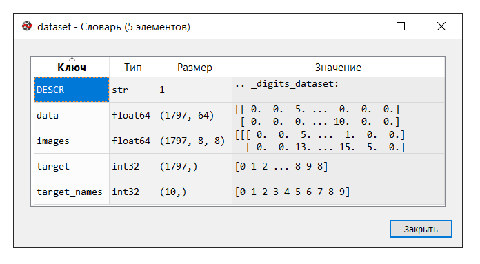
IDE Spyder provides a convenient tool "Variable Manager", which is useful at all times to study machine learning (at least for me), like other "tricks" :
Run the code. In the "variable manager" console, click on the dataset variable. The following dictionary is displayed:
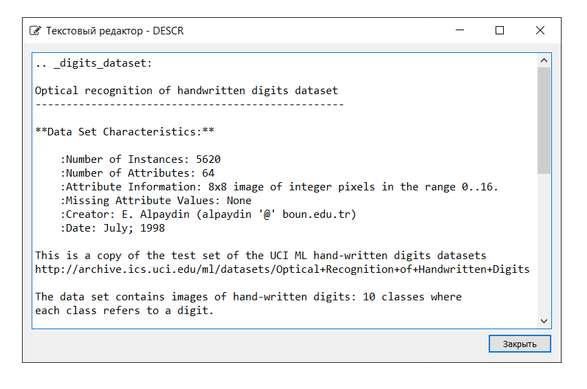
The description of the dataset is as follows:
In this example, we don’t need the 'images' key, so we assign the variable 'data' to the variable X , which is a multidimensional NumPy array with a set of attributes, the size of 1797 rows by 64 columns, and the variable Y to the target, a multidimensional NumPy array with a marker for string.
# # dataset = load_digits() X = dataset.data Y = dataset.target
Next, we divide the data set into the training and test parts, configure the parameters for evaluating the algorithms (cross-validation is used [ one , two ]), defining the metric 'accuracy' in the parameter 'scoring' [ link ]. Accuracy is the proportion of correctly classified objects relative to the total number of objects. The closer the result is to 1, the better [ link ]. Moreover, in one of the books it was found that the results from 0.95 (or 95%) and higher are considered excellent.
# test_size = 0.2 seed = 7 X_train, X_test, Y_train, Y_test = train_test_split(X, Y, test_size=test_size, random_state=seed) # num_folds = 10 n_estimators = 100 scoring = 'accuracy'
Let the variables X_train and Y_train be used for training purposes, X_test and Y_test for the development of forecast values. At the same time, the Y_test variable does not participate in the calculation of the forecast: using the 'score' method, which is the same for each of the algorithms presented below, we will calculate the correct answers using the 'accuracy' metric. This will allow us to judge how the algorithm copes with the task. I do not argue, on our part it is so humanly vile not to prompt the car with the correct answers, but how else to check its performance?
Below is a list of algorithms that we feed the data set with. Based on the results of the calculations, we will conclude which algorithm (which of the algorithms) shows the greatest efficiency. This method may well be called “blitz verification of machine learning algorithms” (hereinafter - blitz verification).
For the convenience of information output, an abbreviation will be affixed next to each algorithm. It should be noted that the settings of each algorithm are accepted by default (default), with the exception of some points, in order to provide equal conditions.
Linear Algorithms:
- Logistic Regression * / Logistic Regression ('LR')
* The word "regression" can be confusing. But do not forget that “Logistic Regression” is a classification algorithm
- Linear Discriminant Analysis ('LDA')
Nonlinear Algorithms:
- Method of k-nearest neighbors (classification) / K-Neighbors Classifier ('KNN')
- Decision Tree Classifier ('CART')
- Naive Bayes Classifier ('NB')
- Linear Support Vector Classification Method (Classification) / Linear Support Vector Classification ('LSVC')
- Support Vector Method (Classification) / C-Support Vector Classification ('SVC')
Artificial Neural Network Algorithm:
- Multilayer Perceptron / Multilayer Perceptrons ('MLP')
Ensemble Algorithms:
- Bagging (classification) / Bagging Classifier ('BG') (Bagging = Bootstrap aggregating)
- Random Forest Classification ('RF')
- Extra Trees Classifier ('ET')
- AdaBoost (classification) / AdaBoost Classifier ('AB') (AdaBoost = Adaptive Boosting)
- Gradient boosting (classification) / Gradient Boosting Classifier ('GB')
Thus, the list of 'models' contains the following models:
models = [] models.append(('LR', LogisticRegression())) models.append(('LDA', LinearDiscriminantAnalysis())) models.append(('KNN', KNeighborsClassifier())) models.append(('CART', DecisionTreeClassifier())) models.append(('NB', GaussianNB())) models.append(('LSVC', LinearSVC())) models.append(('SVC', SVC())) models.append(('MLP', MLPClassifier())) models.append(('BG', BaggingClassifier(n_estimators=n_estimators))) models.append(('RF', RandomForestClassifier(n_estimators=n_estimators))) models.append(('ET', ExtraTreesClassifier(n_estimators=n_estimators))) models.append(('AB', AdaBoostClassifier(n_estimators=n_estimators, algorithm='SAMME'))) models.append(('GB', GradientBoostingClassifier(n_estimators=n_estimators)))
As already mentioned, the effectiveness of each algorithm is evaluated using cross-validation. As a result, a message is displayed (msg - abbreviation from message) containing the following information: model name in the form of an abbreviation, average score of 10-times cross-validation on training data (metric 'accuracy'), standard deviation is shown in brackets , as well as the value of the 'accuracy' metric on the test data.
# scores = [] names = [] results = [] predictions = [] msg_row = [] for name, model in models: kfold = KFold(n_splits=num_folds, random_state=seed) cv_results = cross_val_score(model, X_train, Y_train, cv=kfold, scoring=scoring) names.append(name) results.append(cv_results) m_fit = model.fit(X_train, Y_train) m_predict = model.predict(X_test) predictions.append(m_predict) m_score = model.score(X_test, Y_test) scores.append(m_score) msg = "%s: train = %.3f (%.3f) / test = %.3f" % (name, cv_results.mean(), cv_results.std(), m_score) msg_row.append(msg) print(msg)
After running the code, we get the following results:
LR: train = 0.957 (0.014) / test = 0.948 LDA: train = 0.951 (0.014) / test = 0.946 KNN: train = 0.985 (0.013) / test = 0.981 CART: train = 0.843 (0.033) / test = 0.830 NB: train = 0.819 (0.048) / test = 0.806 LSVC: train = 0.942 (0.017) / test = 0.928 SVC: train = 0.343 (0.079) / test = 0.342 MLP: train = 0.972 (0.012) / test = 0.961 BG: train = 0.952 (0.021) / test = 0.941 RF: train = 0.968 (0.017) / test = 0.965 ET: train = 0.980 (0.010) / test = 0.975 AB: train = 0.827 (0.049) / test = 0.823 GB: train = 0.964 (0.013) / test = 0.968
Span chart ( “box with mustache” ) (box-and-whiskers diagram or plot, box plot):
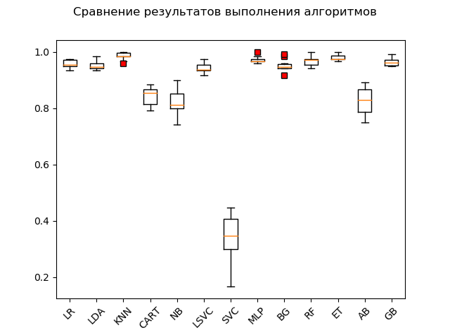
As a result of a blitz test on “raw” data, it can be seen that the algorithms 'KNN' (k-nearest neighbors), 'ET' (extra trees), 'GB' (gradient “boosting”) showed the highest efficiency on the test data, 'RF' (random forest) and 'MLP' (multilayer perceptron):
KNN: train = 0.985 (0.013) / test = 0.981 ET: train = 0.980 (0.010) / test = 0.975 GB: train = 0.964 (0.013) / test = 0.968 RF: train = 0.968 (0.017) / test = 0.965 MLP: train = 0.972 (0.012) / test = 0.961 LR: train = 0.957 (0.014) / test = 0.948 LDA: train = 0.951 (0.014) / test = 0.946 BG: train = 0.952 (0.021) / test = 0.941 LSVC: train = 0.942 (0.017) / test = 0.928 CART: train = 0.843 (0.033) / test = 0.830 AB: train = 0.827 (0.049) / test = 0.823 NB: train = 0.819 (0.048) / test = 0.806 SVC: train = 0.343 (0.079) / test = 0.342
However, many algorithms are very picky about the data that they are served. Therefore, one of the necessary steps is the so-called preliminary data preparation (data pre-processing [ link ])
However, it happens that the algorithm shows the best results without preliminary processing. Hence the following recommendation: include in the blitz test several transformations of the original data set and, after performing the calculations, compare the results in order to catch the essence of the problem as a whole.
The most commonly used methods of preliminary data preparation are:
- standardization;
- scaling (the default range is [0, 1]);
- normalization
These operations with subsequent evaluation can be automated and put on the conveyor using the Pipeline tool.
A code snippet with standardization of the source data is as follows:
# - # ( StandardScaler) pipelines = [] pipelines.append(('SS_LR', Pipeline([('Scaler', StandardScaler()), ('LR', LogisticRegression())]))) pipelines.append(('SS_LDA', Pipeline([('Scaler', StandardScaler()), ('LDA', LinearDiscriminantAnalysis())]))) pipelines.append(('SS_KNN', Pipeline([('Scaler', StandardScaler()), ('KNN', KNeighborsClassifier())]))) pipelines.append(('SS_CART', Pipeline([('Scaler', StandardScaler()), ('CART', DecisionTreeClassifier())]))) pipelines.append(('SS_NB', Pipeline([('Scaler', StandardScaler()), ('NB', GaussianNB())]))) pipelines.append(('SS_LSVC', Pipeline([('Scaler', StandardScaler()), ('LSVC', LinearSVC())]))) pipelines.append(('SS_SVC', Pipeline([('Scaler', StandardScaler()), ('SVC', SVC())]))) pipelines.append(('SS_MLP', Pipeline([('Scaler', StandardScaler()), ('MLP', MLPClassifier())]))) pipelines.append(('SS_BG', Pipeline([('Scaler', StandardScaler()), ('BG', BaggingClassifier(n_estimators=n_estimators))]))) pipelines.append(('SS_RF', Pipeline([('Scaler', StandardScaler()), ('RF', RandomForestClassifier(n_estimators=n_estimators))]))) pipelines.append(('SS_ET', Pipeline([('Scaler', StandardScaler()), ('ET', ExtraTreesClassifier(n_estimators=n_estimators))]))) pipelines.append(('SS_AB', Pipeline([('Scaler', StandardScaler()), ('AB', AdaBoostClassifier(n_estimators=n_estimators, algorithm='SAMME'))]))) pipelines.append(('SS_GB', Pipeline([('Scaler', StandardScaler()), ('GB', GradientBoostingClassifier(n_estimators=n_estimators))]))) # scores_SS = [] names_SS = [] results_SS = [] predictions_SS = [] msg_SS = [] for name, model in pipelines: kfold = KFold(n_splits=num_folds, random_state=seed) cv_results = cross_val_score(model, X_train, Y_train, cv=kfold) names_SS.append(name) results_SS.append(cv_results) m_fit = model.fit(X_train, Y_train) m_predict = model.predict(X_test) predictions_SS.append(m_predict) m_score = model.score(X_test, Y_test) scores_SS.append(m_score) msg = "%s: train = %.3f (%.3f) / test = %.3f" % (name, cv_results.mean(), cv_results.std(), m_score) msg_SS.append(msg) print(msg) # (StandardScaler) fig = pyplot.figure() fig.suptitle(' . ') ax = fig.add_subplot(111) red_square = dict(markerfacecolor='r', marker='s') pyplot.boxplot(results_SS, flierprops=red_square) ax.set_xticklabels(names_SS, rotation=45) pyplot.show()
Note the addition of '_SS' (short for StandardScaler) to list names. This is done in order not to pile up the results, as well as to conveniently view them using the "variable manager" after the conversions are performed.
Running a code snippet produces the following results:
SS_LR: train = 0.958 (0.015) / test = 0.949 SS_LDA: train = 0.951 (0.014) / test = 0.946 SS_KNN: train = 0.968 (0.023) / test = 0.970 SS_CART: train = 0.853 (0.036) / test = 0.835 SS_NB: train = 0.756 (0.046) / test = 0.751 SS_LSVC: train = 0.945 (0.018) / test = 0.941 SS_SVC: train = 0.976 (0.015) / test = 0.990 SS_MLP: train = 0.976 (0.012) / test = 0.973 SS_BG: train = 0.947 (0.018) / test = 0.948 SS_RF: train = 0.973 (0.016) / test = 0.970 SS_ET: train = 0.980 (0.012) / test = 0.975 SS_AB: train = 0.827 (0.049) / test = 0.823 SS_GB: train = 0.964 (0.013) / test = 0.968
Mustache Box (StandardScaler):
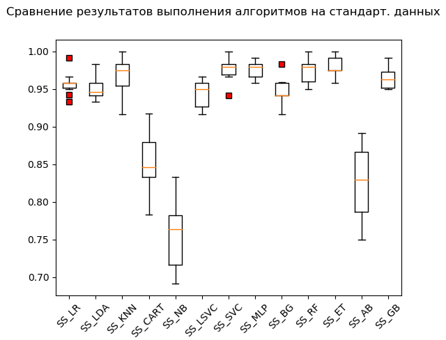
Based on the results of the calculation on standardized data, the following algorithms became leaders:
SS_SVC: train = 0.976 (0.015) / test = 0.990 SS_ET: train = 0.980 (0.012) / test = 0.975 SS_MLP: train = 0.976 (0.012) / test = 0.973 SS_KNN: train = 0.968 (0.023) / test = 0.970 SS_RF: train = 0.973 (0.016) / test = 0.970 SS_GB: train = 0.964 (0.013) / test = 0.968 SS_LR: train = 0.958 (0.015) / test = 0.949 SS_BG: train = 0.947 (0.018) / test = 0.948 SS_LDA: train = 0.951 (0.014) / test = 0.946 SS_LSVC: train = 0.945 (0.018) / test = 0.941 SS_CART: train = 0.853 (0.036) / test = 0.835 SS_AB: train = 0.827 (0.049) / test = 0.823 SS_NB: train = 0.756 (0.046) / test = 0.751
As they say, from rags to riches: the support vector method ('SVC'), fed by standardized data, did the rest, showing an excellent result. During the “manual” check, comparing the values of the variables Y_test and predictions_SS [6] , the algorithm did not chew only a few values.
The following code is executed for the functions MinMaxScaler (scaling) and Normalizer (normalization). I will not give the full code in the article. You can download it from my GitHub repository: link .
Just do not forget to hang for a while and laugh at yourself at 'for educational purpose only'! :)
As a result, after going through the entire code, we get the following results:
LR: train = 0.957 (0.014) / test = 0.948 LDA: train = 0.951 (0.014) / test = 0.946 KNN: train = 0.985 (0.013) / test = 0.981 CART: train = 0.843 (0.033) / test = 0.830 NB: train = 0.819 (0.048) / test = 0.806 LSVC: train = 0.942 (0.017) / test = 0.928 SVC: train = 0.343 (0.079) / test = 0.342 MLP: train = 0.972 (0.012) / test = 0.961 BG: train = 0.952 (0.021) / test = 0.941 RF: train = 0.968 (0.017) / test = 0.965 ET: train = 0.980 (0.010) / test = 0.975 AB: train = 0.827 (0.049) / test = 0.823 GB: train = 0.964 (0.013) / test = 0.968 SS_LR: train = 0.958 (0.015) / test = 0.949 SS_LDA: train = 0.951 (0.014) / test = 0.946 SS_KNN: train = 0.968 (0.023) / test = 0.970 SS_CART: train = 0.853 (0.036) / test = 0.835 SS_NB: train = 0.756 (0.046) / test = 0.751 SS_LSVC: train = 0.945 (0.018) / test = 0.941 SS_SVC: train = 0.976 (0.015) / test = 0.990 SS_MLP: train = 0.976 (0.012) / test = 0.973 SS_BG: train = 0.947 (0.018) / test = 0.948 SS_RF: train = 0.973 (0.016) / test = 0.970 SS_ET: train = 0.980 (0.012) / test = 0.975 SS_AB: train = 0.827 (0.049) / test = 0.823 SS_GB: train = 0.964 (0.013) / test = 0.968 MMS_LR: train = 0.961 (0.013) / test = 0.953 MMS_LDA: train = 0.951 (0.014) / test = 0.946 MMS_KNN: train = 0.985 (0.013) / test = 0.981 MMS_CART: train = 0.850 (0.027) / test = 0.840 MMS_NB: train = 0.796 (0.045) / test = 0.786 MMS_LSVC: train = 0.964 (0.012) / test = 0.958 MMS_SVC: train = 0.963 (0.016) / test = 0.956 MMS_MLP: train = 0.972 (0.011) / test = 0.963 MMS_BG: train = 0.948 (0.024) / test = 0.946 MMS_RF: train = 0.973 (0.014) / test = 0.968 MMS_ET: train = 0.983 (0.010) / test = 0.981 MMS_AB: train = 0.827 (0.049) / test = 0.823 MMS_GB: train = 0.963 (0.013) / test = 0.968 N_LR: train = 0.938 (0.020) / test = 0.919 N_LDA: train = 0.952 (0.013) / test = 0.949 N_KNN: train = 0.981 (0.012) / test = 0.985 N_CART: train = 0.834 (0.028) / test = 0.825 N_NB: train = 0.825 (0.043) / test = 0.805 N_LSVC: train = 0.960 (0.014) / test = 0.953 N_SVC: train = 0.551 (0.053) / test = 0.586 N_MLP: train = 0.963 (0.018) / test = 0.946 N_BG: train = 0.949 (0.016) / test = 0.938 N_RF: train = 0.973 (0.015) / test = 0.970 N_ET: train = 0.982 (0.012) / test = 0.980 N_AB: train = 0.825 (0.040) / test = 0.820 N_GB: train = 0.953 (0.022) / test = 0.956
'Top 5' results:
SS_SVC: train = 0.976 (0.015) / test = 0.990 N_KNN: train = 0.981 (0.012) / test = 0.985 KNN: train = 0.985 (0.013) / test = 0.981 MMS_KNN: train = 0.985 (0.013) / test = 0.981 MMS_ET: train = 0.983 (0.010) / test = 0.981
Thus, according to the results of a blitz test of machine learning algorithms to solve the classification problem of the 'digits' dataset, the most suitable machine learning algorithms are: the k-nearest neighbors ('KNN') method, the support vector method ('SVC') and extra-trees ('ET'). These algorithms should be paid closer attention to the further development of results aimed at increasing the efficiency of calculations. Everything, as they say, is solvable.
And on this raised note, smoothly proceed to the 2nd part.
Forecasting problem
We move on the thumb:
# from sklearn.datasets import load_boston from sklearn.model_selection import train_test_split from sklearn.linear_model import LinearRegression from sklearn.linear_model import Ridge from sklearn.linear_model import Lasso from sklearn.linear_model import ElasticNet from sklearn.linear_model import LarsCV from sklearn.linear_model import BayesianRidge from sklearn.neighbors import KNeighborsRegressor from sklearn.tree import DecisionTreeRegressor from sklearn.svm import LinearSVR from sklearn.svm import SVR from sklearn.ensemble import AdaBoostRegressor from sklearn.ensemble import BaggingRegressor from sklearn.ensemble import ExtraTreesRegressor from sklearn.ensemble import GradientBoostingRegressor from sklearn.ensemble import RandomForestRegressor from sklearn.model_selection import KFold from sklearn.model_selection import cross_val_score from sklearn.pipeline import Pipeline from sklearn.preprocessing import StandardScaler from sklearn.preprocessing import Normalizer from matplotlib import pyplot # dataset = load_boston()
Run the code and deal with the dictionary. Description and keys are as follows:


We assign the key 'data' to the variable X , which is a multidimensional NumPy array with a set of attributes, dimension 506 rows by 13 columns, and the variable Y - 'target', a multidimensional NumPy array with a marker for each row.
# #dataset = load_boston() X = dataset.data Y = dataset.target
We divide the data set into training and test parts, configure the parameters for evaluating the algorithms. In the parameter 'scoring' we set one of the metrics 'r2' traditional for regression analysis:
# dataset = load_boston() X = dataset.data Y = dataset.target # test_size = 0.2 seed = 7 X_train, X_test, Y_train, Y_test = train_test_split(X, Y, test_size=test_size, random_state=seed) # num_folds = 10 n_iter = 1000 n_estimators = 100 scoring = 'r2'
R2 - coefficient of determination - this is the proportion of the variance of the dependent variable, explained by the model in question ( link ).
“The coefficient of determination for a model with a constant takes values from 0 to 1. The closer the coefficient is to 1, the stronger the dependence. When evaluating regression models, this is interpreted as matching the model with data. For acceptable models, it is assumed that the coefficient of determination should be at least at least 50% (in this case, the coefficient of multiple correlation exceeds 70% modulo). Models with a determination coefficient above 80% can be considered quite good (the correlation coefficient exceeds 90%). The equality of the determination coefficient to unity means that the explained variable is exactly described by the model under consideration ” (ibid.).
To solve the forecasting problem, we use the following algorithms:
Linear Algorithms:
- Linear Regression ('LR')
- Ridge regression (ridge regression) / Ridge Regression ('R')
- Lasso regression (from English LASSO - Least Absolute Shrinkage and Selection Operator) / Lasso Regression ('L')
- Elastic Net Regression ('ELN') regression method
- Least Angle Regression (LARS) ('LARS') method
- Bayesian ridge regression / Bayesian ridge regression ('BR')
Nonlinear Algorithms:
- k-nearest neighbors regressor ('KNR') method
- Decision Tree Regressor ('DTR')
- Linear Support Vector Machine (regression) / Linear Support Vector Machine - Regression / ('LSVR')
- Support Vector Method (Regression) / Epsilon-Support Vector Regression ('SVR')
Ensemble Algorithms:
- AdaBoost (regression) / AdaBoost Regressor ('ABR') (AdaBoost = Adaptive Boosting)
- Bagging (regression) / Bagging Regressor ('BR') (Bagging = Bootstrap aggregating)
- Extra Trees Regressor ('ETR')
- Gradient boosting (regression) / Gradient Boosting Regressor ('GBR')
- Random Forest Classification (regression) / Random Forest Classifier ('RFR')
Thus, the list of 'models' contains the following models:
models = [] models.append(('LR', LinearRegression())) models.append(('R', Ridge())) models.append(('L', Lasso())) models.append(('ELN', ElasticNet())) models.append(('LARS', Lars())) models.append(('BR', BayesianRidge(n_iter=n_iter))) models.append(('KNR', KNeighborsRegressor())) models.append(('DTR', DecisionTreeRegressor())) models.append(('LSVR', LinearSVR())) models.append(('SVR', SVR())) models.append(('ABR', AdaBoostRegressor(n_estimators=n_estimators))) models.append(('BR', BaggingRegressor(n_estimators=n_estimators))) models.append(('ETR', ExtraTreesRegressor(n_estimators=n_estimators))) models.append(('GBR', GradientBoostingRegressor(n_estimators=n_estimators))) models.append(('RFR', RandomForestRegressor(n_estimators=n_estimators)))
As with classification, evaluating the effectiveness of each algorithm is done using cross-validation. The displayed message contains the following information: the name of the model in the form of an abbreviation, the average score of a 10-fold cross-validation on training data (metric 'r2'), the standard deviation and the coefficient of determination r2 on test data are shown in brackets.
# scores = [] names = [] results = [] predictions = [] msg_row = [] for name, model in models: kfold = KFold(n_splits=num_folds, random_state=seed) cv_results = cross_val_score(model, X_train, Y_train, cv=kfold, scoring=scoring) names.append(name) results.append(cv_results) m_fit = model.fit(X_train, Y_train) m_predict = model.predict(X_test) predictions.append(m_predict) m_score = model.score(X_test, Y_test) scores.append(m_score) msg = "%s: train = %.3f (%.3f) / test = %.3f" % (name, cv_results.mean(), cv_results.std(), m_score) msg_row.append(msg) print(msg) # (« ») fig = pyplot.figure() fig.suptitle(' ') ax = fig.add_subplot(111) red_square = dict(markerfacecolor='r', marker='s') pyplot.boxplot(results, flierprops=red_square) ax.set_xticklabels(names, rotation=45) pyplot.show()
After running the code, we get the following results:
LR: train = 0.746 (0.068) / test = 0.579 R: train = 0.744 (0.067) / test = 0.570 L: train = 0.689 (0.070) / test = 0.641 ELN: train = 0.677 (0.074) / test = 0.662 LARS: train = 0.744 (0.069) / test = 0.579 BR: train = 0.739 (0.069) / test = 0.571 KNR: train = 0.434 (0.288) / test = 0.538 DTR: train = 0.671 (0.145) / test = 0.637 LSVR: train = 0.550 (0.144) / test = 0.459 SVR: train = -0.012 (0.048) / test = -0.003 ABR: train = 0.810 (0.078) / test = 0.763 BR: train = 0.854 (0.064) / test = 0.805 ETR: train = 0.889 (0.047) / test = 0.836 GBR: train = 0.878 (0.042) / test = 0.863 RFR: train = 0.852 (0.068) / test = 0.819
Span Chart:
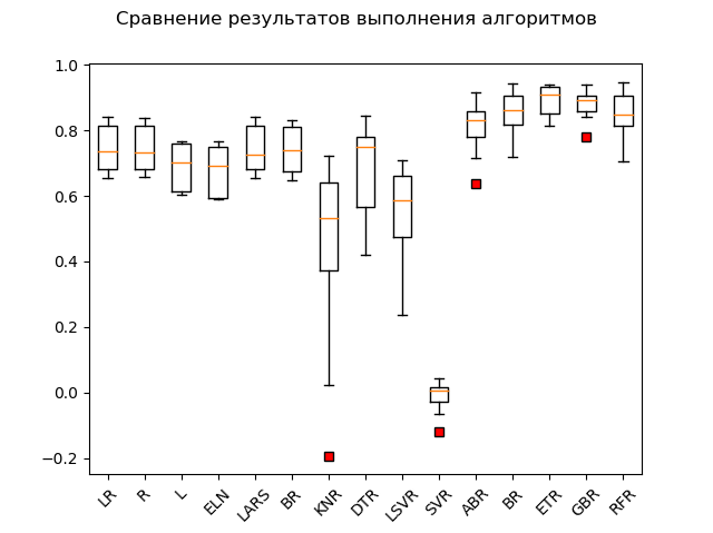
The obvious leaders are the ensemble methods 'GBR' (gradient 'boosting'), 'ETR' (extra-trees), 'RFR' (random forest) and 'BR' ('bagging'):
GBR: train = 0.878 (0.042) / test = 0.863 ETR: train = 0.889 (0.047) / test = 0.836 RFR: train = 0.852 (0.068) / test = 0.819 BR: train = 0.854 (0.064) / test = 0.805 ABR: train = 0.810 (0.078) / test = 0.763 ELN: train = 0.677 (0.074) / test = 0.662 L: train = 0.689 (0.070) / test = 0.641 DTR: train = 0.671 (0.145) / test = 0.637 LR: train = 0.746 (0.068) / test = 0.579 LARS: train = 0.744 (0.069) / test = 0.579 BR: train = 0.739 (0.069) / test = 0.571 R: train = 0.744 (0.067) / test = 0.570 KNR: train = 0.434 (0.288) / test = 0.538 LSVR: train = 0.550 (0.144) / test = 0.459 SVR: train = -0.012 (0.048) / test = -0.003
One "adabust", "loshara" sort of, lags behind.
Perhaps the three leaders are combing standardization and normalization. Let's find out by executing the rest of the code.
The results are as follows:
SS_LR: train = 0.746 (0.068) / test = 0.579 SS_R: train = 0.746 (0.068) / test = 0.578 SS_L: train = 0.678 (0.054) / test = 0.510 SS_ELN: train = 0.665 (0.060) / test = 0.513 SS_LARS: train = 0.744 (0.069) / test = 0.579 SS_BR: train = 0.746 (0.066) / test = 0.576 SS_KNR: train = 0.763 (0.098) / test = 0.739 SS_DTR: train = 0.610 (0.242) / test = 0.629 SS_LSVR: train = 0.727 (0.091) / test = 0.482 SS_SVR: train = 0.653 (0.126) / test = 0.610 SS_ABR: train = 0.811 (0.076) / test = 0.819 SS_BR: train = 0.853 (0.074) / test = 0.813 SS_ETR: train = 0.887 (0.048) / test = 0.846 SS_GBR: train = 0.878 (0.038) / test = 0.860 SS_RFR: train = 0.851 (0.071) / test = 0.818 N_LR: train = 0.751 (0.099) / test = 0.576 N_R: train = 0.287 (0.126) / test = 0.271 N_L: train = -0.030 (0.032) / test = -0.000 N_ELN: train = -0.007 (0.030) / test = 0.023 N_LARS: train = 0.751 (0.099) / test = 0.576 N_BR: train = 0.744 (0.100) / test = 0.589 N_KNR: train = 0.485 (0.192) / test = 0.504 N_DTR: train = 0.729 (0.080) / test = 0.765 N_LSVR: train = 0.182 (0.108) / test = 0.136 N_SVR: train = 0.086 (0.076) / test = 0.084 N_ABR: train = 0.795 (0.053) / test = 0.752 N_BR: train = 0.854 (0.054) / test = 0.827 N_ETR: train = 0.877 (0.048) / test = 0.850 N_GBR: train = 0.852 (0.063) / test = 0.872 N_RFR: train = 0.852 (0.051) / test = 0.801
As you can see, ensemble methods are still ahead of everyone.
'Top 5' contains the following results:
N_GBR: train = 0.852 (0.063) / test = 0.872 GBR: train = 0.878 (0.042) / test = 0.863 SS_GBR: train = 0.878 (0.038) / test = 0.860 N_ETR: train = 0.877 (0.048) / test = 0.850 SS_ETR: train = 0.887 (0.048) / test = 0.846
We will display a chart comparing the results:
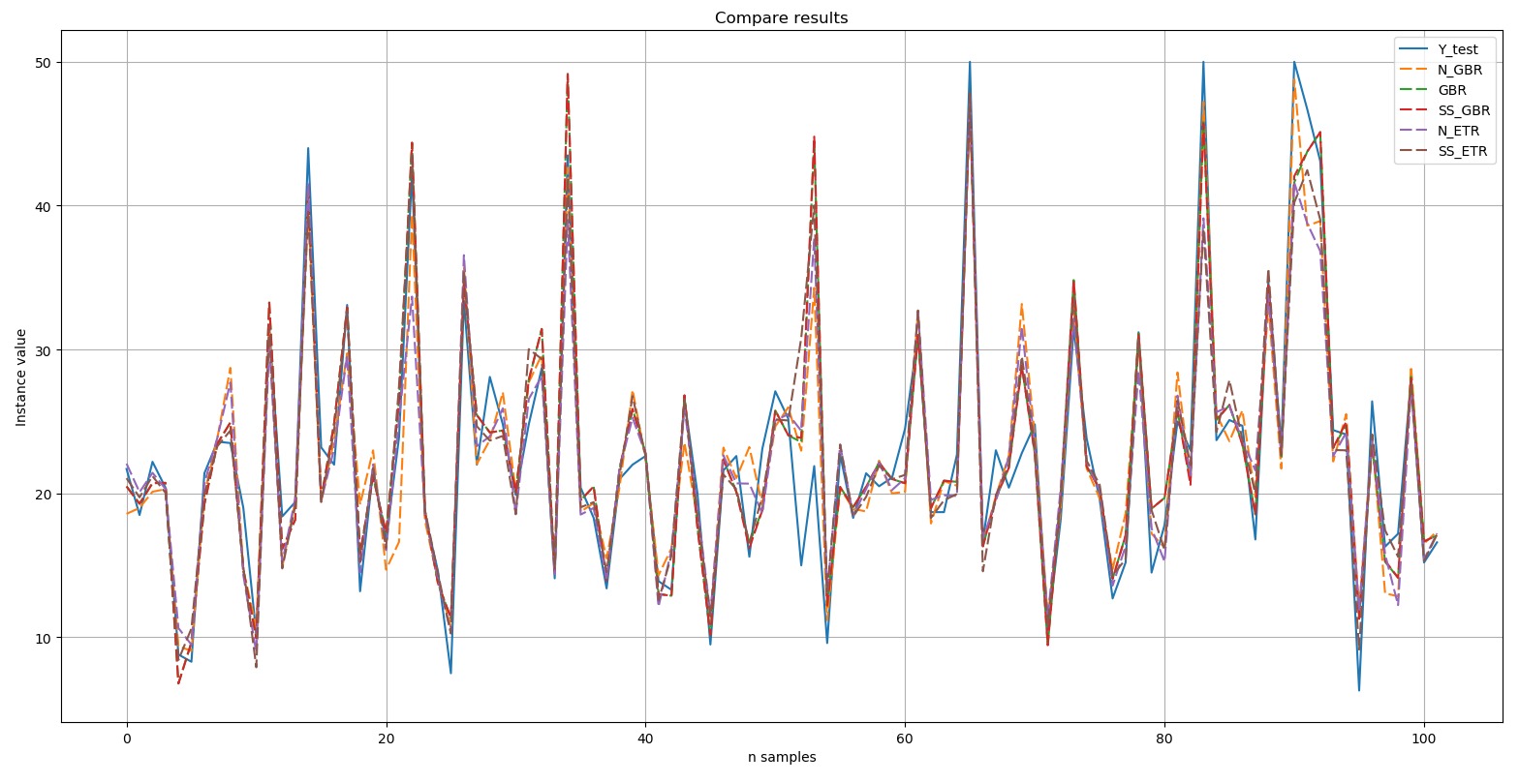
Y-test is the standard. The five selected results presented in the diagram are indicated by a dashed line. It can be seen that all the peaks were reproduced either with exact repetition, or to one degree or another.
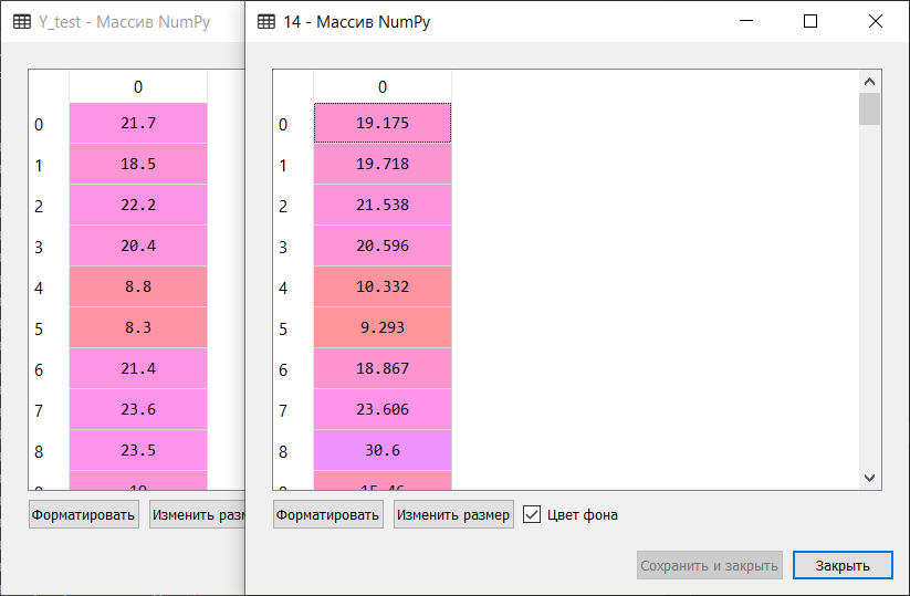
Short excerpt of manual comparison of reference values and forecast values of the algorithm included in Top 5:
Thus, according to the results of a blitz-test of machine learning algorithms to solve the problem of predicting the 'boston house-price' dataset, the most suitable algorithms are gradient “boosting” ('GBR ') and extra trees (' ETR '). These algorithms should be paid closer attention to further develop the results and enhance the effectiveness of forecasts.
Afterword
A quick check of machine learning algorithms allows, to a first approximation, to identify the most effective algorithms for solving problems of classification and regression analysis (forecasting). We were convinced of this by processing the 'digits' dataset, brilliantly sorting the instances into 10 classes, as well as the 'boston house-price' dataset, “amazingly” sorting out finding dependencies and performing a “fluctuating” forecast of the dependent variable.
You are also invited to try this method on your own data sets or on those that you can dig on various repositories, including GitHub. For example: link .
Get a suitable data set for the target - and set a flock of algorithms on it in the team of the blitz test. And there it becomes clear whose take: one in the field is not a warrior. :)
In conclusion. I will be grateful for your comments, questions and suggestions, as the basis of this article is the information that I share with new colleagues on each new project in the field of machine learning. Each of them has its own specialization, about machine learning and artificial neural networks, many of them only “heard somewhere”, so it’s important for me to talk about complex, multifaceted and, finally, impregnable (this is about ANN and machine learning in general) :), in a simple and understandable language; show that it is not the gods who burn the pots; and that if there is interest, then more than a dozen algorithms can be "harnessed". :)
PS By the end of the article I already began to predict myself, so to the upcoming questions about where I got the cheat sheet in the first figure I give out: everything on the same site scikit-learn.org ( 'Choosing the right estimator' ): link . And the personification of artificial intelligence in the form of a blushed Samodelkin is so from the waves of memory of my happy childhood.