Synopsis on “Machine Learning”. Mathematical analysis. Gradient descent

Recall the mathematical analysis

Function Continuity and Derivative

Let $$$E \ subseteq \ mathbb {R}$ , $$$a$ Is the limit point of the set $$$E$ (those. $$$a \ in E, \ forall \ varepsilon> 0 \ space \ space | (a - \ varepsilon, a + \ varepsilon) \ cap E | = \ infty$ ), $$$f \ colon E \ to \ mathbb {R}$ .



Definition 1 (Cauchy function limit):



Function $$$f \ colon E \ to \ mathbb {R}$ committed to $$$A$ at $$$x$ seeking to $$$a$ , if a

$$

$$\ forall \ varepsilon> 0 \ space \ space \ exists \ delta> 0 \ space \ space \ forall x \ in E \ space \ space (0 <| x- a | <\ delta \ Rightarrow | f (x) - A | <\ varepsilon).$$

Designation: $$$\ lim \ limits_ {E \ ni x \ to a} f (x) = A$ .



Definition 2:

1. Interval $$$ab$ called set $$$] a, b [\ space: = \ {x \ in \ mathbb {R} | a <x <b \}$ ;
2. Point Interval $$$x \ in \ mathbb {R}$ is called the neighborhood of this point.
3. A punctured neighborhood of a point is a neighborhood of a point from which this point itself is excluded.

Designation:

1. $$$V (x)$ or $$$U (x)$ - neighborhood of a point $$$x$ ;
2. $$$\ overset {\ circ} {U} (x)$ - punctured neighborhood of a point $$$x$ ;
3. $$$U_E (x): = E \ cap U (x), \\ \ overset {\ circ} {U} _E (x): = E \ cap \ overset {\ circ} {U} (x)$

Definition 3 (function limit through neighborhoods):

$$

$$\ lim \ limits_ {E \ ni x \ to a} f (x) = A: = \ forall V_R (A) \ space \ exists \ overset {\ circ} {U} _E (a) \ space \ space ( f (\ overset {\ circ} {U} _E (a)) \ subset V_R (A)).$$

Definitions 1 and 3 are equivalent.



Definition 4 (continuity of a function at a point):

1. $$$f \ colon E \ to \ mathbb {R}$ continuous in $$$a \ in E: =$
   
   
   
   
   

   $$

   $$= \ forall V (f (a)) \ space \ space \ exists U_E (a) \ space \ space (f (U_E (a)) \ subset V (f (a)));$$
   
   
   
   
   
2. $$$f \ colon E \ to \ mathbb {R}$ continuous in $$$a \ in E: =$
   
   
   
   
   

   $$

   $$\ forall \ varepsilon> 0 \ space \ space \ exists \ delta> 0 \ space \ space \ forall x \ in E \ space \ space (| xa | <\ delta \ Rightarrow | f (x) -f (a) | <\ varepsilon).$$
   
   
   
   
   

Definitions 3 and 4 show that

( $$$f \ colon E \ to \ mathbb {R}$ continuous in $$$a \ in E$ where $$$a$ - limit point $$$E$ ) $$$\ Leftrightarrow$

$$$\ Leftrightarrow (\ lim \ limits_ {E \ ni x \ to a} f (x) = f (a)).$



Definition 5:



Function $$$f \ colon E \ to \ mathbb {R}$ called continuous on the set $$$E$ if it is continuous at each point of the set $$$E$ .



Definition 6:

1. Function $$$f \ colon E \ to \ mathbb {R}$ defined on the set $$$E \ subset \ mathbb {R}$ is called differentiable at the point $$$a \ in E$ limiting for the set $$$E$ if there is such a linear with respect to the increment $$$x-a$ argument function $$$A \ cdot (x-a)$ [function differential $$$f$ at the point $$$a$ ] that increment $$$f (x) -f (a)$ the functions $$$f$ represented as
   
   
   
   
   

   $$

   $$f (x) -f (a) = A \ cdot (x-a) + o (x-a) \ quad for \ space x \ to a, \ space x \ in E.$$
   
   
   
   
   
2. Value
   
   
   
   
   
   
   

   $$

   $$f '(a) = \ lim \ limits_ {E \ ni x \ to a} \ frac {f (x) -f (a)} {x-a}$$
   
   
   
   
   
   
   called derivative function $$$f$ at the point $$$a$ .

Also

$$

$$f '(x) = \ lim _ {\ substack {h \ to 0 \\ x + h, x \ in E}} \ frac {f (x + h) -f (x)} {h}.$$

Definition 7:

1. Dot $$$x_0 \ in E \ subset \ mathbb {R}$ is called the point of local maximum (minimum) , and the value of the function in it is called the local maximum (minimum) of the function $$$f \ colon E \ to \ mathbb {R}$ , if a $$$\ exists U_E (x_0)$ :
   
   
   
   
   

   $$

   $$\ forall x \ in U_E (x_0) \ space \ space f (x) \ leq f (x_0) (respectively, f (x) \ geq f (x_0)).$$
   
   
   
   
   
2. The points of local maximum and minimum are called points of local extremum , and the values ​​of the function in them are called local extrema of the function .
3. Dot $$$x_0 \ in E$ extremum function $$$f \ colon E \ to \ mathbb {R}$ called an internal extremum point if $$$x_0$ is the limit point as for the set $$$E _- = \ {x \ in E | x <x_0 \}$ , and for the set $$$E _ + = \ {x \ in E | x> x_0 \}$ .

Lemma 1 (Fermat):



If the function $$$f \ colon E \ to \ mathbb {R}$ differentiable at the point of internal extremum $$$x_0 \ in E$ , then its derivative at this point is zero: $$$f '(x_0) = 0$ .



Proposition 1 (Roll's theorem):

If the function $$$f \ colon [a, b] \ to \ mathbb {R}$ continuous on a segment $$$[a, b]$ differentiable in the interval $$$] a, b [$ and $$$f (a) = f (b)$ then there is a point $$$\ xi \ in] a, b [$ such that $$$f '(\ xi) = 0$ .



Theorem 1 (Lagrange finite increment theorem):



If the function $$$f \ colon [a, b] \ to \ mathbb {R}$ continuous on a segment $$$[a, b]$ and differentiable in the interval $$$] a, b [$ then there is a point $$$\ xi \ in] a, b [$ such that

$$

$$f (b) -f (a) = f '(\ xi) (b-a).$$

Corollary 1 (a sign of monotonicity of a function):

If at any point of a certain interval the derivative of the function is non-negative (positive), then the function does not decrease (increases) on this interval.



Corollary 2 (criterion for the constancy of a function):

Continuous on a cut $$$[a, b]$ a function is not constant if and only if its derivative is zero at any point in the interval $$$[a, b]$ (or at least the interval $$$] a, b [$ )

Partial derivative of a function of many variables

Across $$$\ mathbb {R} ^ m$ denote the set:

$$

$$\ mathbb {R} ^ m = \ underbrace {\ mathbb {R} \ times \ mathbb {R} \ times \ cdots \ times \ mathbb {R}} _ m = \ {(\ omega_1, \ omega_2, ... , \ omega_m), \ space \ omega_i \ in \ mathbb {R} \ space \ forall i \ in \ overline {1, m} \}.$$

Definition 8:



Function $$$f \ colon E \ to \ mathbb {R}$ defined on the set $$$E \ subset \ mathbb {R} ^ m$ is called differentiable at the point $$$x \ in E$ limiting for the set $$$E$ , if a

$$

$$f (x + h) -f (x) = L (x) h + \ alpha (x; h), \ qquad (1)$$

Where $$$L (x) \ colon \ mathbb {R} ^ m \ to \ mathbb {R}$ - linear with respect to $$$h$ function [function differential $$$f$ at the point $$$x$ (reference $$$df (x)$ or $$$f '(x)$ )], but $$$\ alpha (x; h) = o (h)$ at $$$h \ to 0, x + h \ in E$ .



Relation (1) can be rewritten as follows:

$$

$$f (x + h) -f (x) = f '(x) h + \ alpha (x; h)$$

or

$$

$$\ bigtriangleup f (x; h) = df (x) h + \ alpha (x; h).$$

If we go to the coordinate record of the point $$$x = (x ^ 1, ..., x ^ m)$ , vector $$$h = (h ^ 1, ..., h ^ m)$ and linear function $$$L (x) h = a_1 (x) h ^ 1 + ... + a_m (x) h ^ m$ , then equality (1) looks like this

$$

$$f (x ^ 1 + h ^ 1, ..., x ^ m + h ^ m) -f (x ^ 1, ..., x ^ m) = \\ = a_1 (x) h ^ 1 + ... + a_m (x) h ^ m + o (h) \ quad for \ space \ space h \ to 0, \ qquad (2)$$

Where $$$a_1 (x), ..., a_m (x)$ - associated with point $$$x$ real numbers. You need to find these numbers.



We denote

$$

$$h_i = h ^ ie_i = 0 \ cdot e_1 + ... + 0 \ cdot e_ {i-1} + h ^ i \ cdot e_i + 0 \ cdot e_ {i + 1} + ... + 0 \ cdot e_m,$$

Where $$$\ {e_1, ..., e_m \}$ - basis in $$$\ mathbb {R} ^ m$ .



At $$$h = h_i$ from (2) we obtain

$$

$$f (x ^ 1, ..., x ^ {i-1}, x ^ i + h ^ i, x ^ {i + 1}, ..., x ^ m) -f (x ^ 1, ..., x ^ i, ..., x ^ m) = \\ = a_i (x) h ^ i + o (h ^ i) \ quad for \ space \ space h ^ i \ to 0. \ qquad (3)$$

From (3) we obtain

$$

$$a_i (x) = \ lim_ {h_i \ to 0} \ frac {f (x ^ 1, ..., x ^ {i-1}, x ^ i + h ^ i, x ^ {i + 1} , .., x ^ m) -f (x ^ 1, ..., x ^ i, ..., x ^ m)} {h ^ i}. \ qquad (4)$$

Definition 9:

The limit (4) is called the partial derivative of the function $$$f (x)$ at the point $$$x = (x ^ 1, ..., x ^ m)$ by variable $$$x ^ i$ . It is designated:

$$

$$\ frac {\ partial f} {\ partial x ^ i} (x), \ quad \ partial_if (x), \ quad f '_ {x ^ i} (x).$$

Example 1:

$$

$$f (u, v) = u ^ 3 + v ^ 2 \ sin u, \\ \ partial_1f (u, v) = \ frac {\ partial f} {\ partial u} (u, v) = 3u ^ 2 + v ^ 2 \ cos u, \\ \ partial_2 f (u, v) = \ frac {\ partial f} {\ partial v} (u, v) = 2v \ sin u.$$

Gradient descent

Let $$$f \ colon \ mathbb {R} ^ n \ to \ mathbb {R}$ where $$$\ mathbb {R} ^ n = \ underbrace {\ mathbb {R} \ times \ mathbb {R} \ times \ cdots \ times \ mathbb {R}} _ n = \ {(\ theta_1, \ theta_2, ... , \ theta_n), \ space \ theta_i \ in \ mathbb {R} \ space \ forall i \ in \ overline {1, n} \}$ .



Definition 10:



Gradient Function $$$f \ colon \ mathbb {R} ^ n \ to \ mathbb {R}$ called a vector, $$$i$ whose element is equal to $$$\ frac {\ partial f} {\ partial \ theta_i}$ :

$$

$$\ bigtriangledown _ {\ theta} f = \ left (\ begin {array} {c} \ frac {\ partial f} {\ partial \ theta_1} \\\ frac {\ partial f} {\ partial \ theta_2} \\ \ vdots \\\ frac {\ partial f} {\ partial \ theta_n} \ end {array} \ right), \ quad \ theta = (\ theta_1, \ theta_2, ..., \ theta_n).$$

Gradient is the direction in which the function increases most rapidly. This means that the direction in which it decreases most rapidly is the direction opposite to the gradient, i.e. $$$- \ bigtriangledown _ {\ theta} f$ .



The aim of the gradient descent method is to find the extremum (minimum) point of the function.



Denote by $$$\ theta ^ {(t)}$ function parameter vector in step $$$t$ . Parameter update vector in step $$$t$ :

$$

$$u ^ {(t)} = - \ eta \ bigtriangledown _ {\ theta} f (\ theta ^ {(t-1)}), \ quad \ theta ^ {(t)} = \ theta ^ {(t- 1)} + u ^ {(t)}.$$

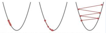
In the formula above, the parameter $$$\ eta$ Is the learning speed that controls the size of the step that we take in the direction of the gradient slope. In particular, two opposing problems may arise:

• if the steps are too small, the training will be too long, and the likelihood of getting stuck in a small unsuccessful local minimum along the road increases (the first image in the picture below);
• if they are too large, you can endlessly jump over the desired minimum back and forth, but never reach the lowest point (the third image in the picture below).

Example:

Consider the example of the gradient descent method in the simplest case ( $$$n = 1$ ) I.e $$$f \ colon \ mathbb {R} \ to \ mathbb {R}$ .

Let $$$f (x) = x ^ 2, \ quad \ theta ^ {(0)} = 3, \ quad \ eta = 1$ . Then:

$$

$$\ frac {\ partial f} {\ partial x} (x) = 2x \ quad \ Rightarrow \ quad \ bigtriangledown f_ \ theta (x) = 2x; \\ \ theta ^ {(1)} = \ theta ^ {(0)} - 1 \ cdot f_ \ theta (\ theta ^ {(0)}) = 3 - 6 = -3; \\ \ theta ^ {(2)} = \ theta ^ {(1)} - 1 \ cdot f_ \ theta (\ theta ^ {(1)}) = - 3 + 6 = 3 = \ theta ^ {(0 )}.$$

In the case when $$$\ eta = 1$ , the situation turns out, as in the third image of the picture above. We constantly jump over the extreme point.

Let $$$\ eta = 0.8$ . Then:

$$

$$\ theta ^ {(1)} = \ theta ^ {(0)} - 0.8 \ times f_ \ theta (\ theta ^ {(0)}) = 3 - 0.8 \ times6 = 3 - 4.8 = -1.8; \\ \ theta ^ {(2)} = \ theta ^ {(1)} - 0.8 \ times f_ \ theta (\ theta ^ {(1)}) = - 1.8 + 0.8 \ times3.6 = -1.8 + 2.88 = 1.08; \\ \ theta ^ {(3)} = \ theta ^ {(2)} - 0.8 \ times f_ \ theta (\ theta ^ {(2)}) = 1.08 - 0.8 \ times2.16 = 1.08 - 1.728 = - 0.648; \\ \ theta ^ {(4)} = \ theta ^ {(3)} - 0.8 \ times f_ \ theta (\ theta ^ {(3)}) = - 0.648 + 0.8 \ times1.296 = -0.648 + 1.0368 = 0.3888; \\ \ theta ^ {(5)} = \ theta ^ {(4)} - 0.8 \ times f_ \ theta (\ theta ^ {(4)}) = 0.3888 - 0.8 \ times0.7776 = 0.3888 - .62208 = -0.23328; \\ \ theta ^ {(6)} = \ theta ^ {(5)} - 0.8 \ times f_ \ theta (\ theta ^ {(5)}) = - 0.23328 + 0.8 \ times0.46656 = -0.23328 + 0.373248 = \\ = 0.139968.$$

It is seen that iteratively we are approaching the point of extremum.

Let $$$\ eta = 0.5$ . Then:

$$

$$\ theta ^ {(1)} = \ theta ^ {(0)} - 0.5 \ times f_ \ theta (\ theta ^ {(0)}) = 3 - 0.5 \ times6 = 3 - 3 = 0; \\ \ theta ^ {(2)} = \ theta ^ {(1)} - 0.5 \ times f_ \ theta (\ theta ^ {(1)}) = 0 - 0.5 \ times0 = 0.$$

The extremum point was found in 1 step.

Bibliography:

• "Mathematical analysis. Part 1 ", V.A. Zorich, Moscow, 1997;
• “Deep learning. Immersion in the world of neural networks ”, S. Nikulenko, A. Kadurin, E. Arkhangelskaya, PETER, 2018.