😵 👩‍👦‍👦 🔲 Julia and Neural Networks: Flux 🐲 👏🏼 ♌️

A little over a year has passed since MIT announced the release of the high-performance general-purpose language Julia . Since then, the language has gained popularity: it is used in more than 1,500 universities (in some it is taught as the first language of instruction), and the fields of application cover from medical diagnostics and space mission planning to pressing problems such as optimizing school bus traffic .

One of the key fields of activity of many projects, as you might guess, is machine learning, for which Julia has many powerful tools , and a rather interesting project has recently been published - General Probability Programming System "GEN" .

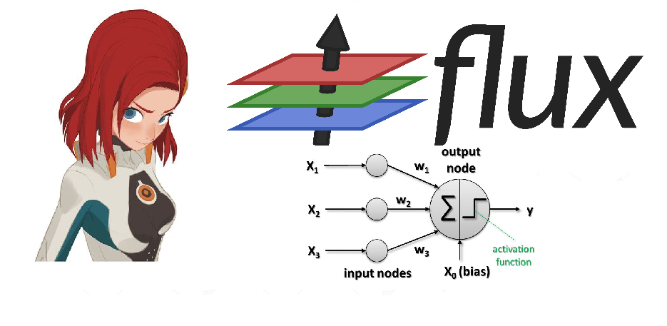
Today we will pay attention to, as the name implies, the Flux package, which provides all the power of neural networks. We will try to go from processing and researching sets of images to a trained neural network to get a full classifier!

Official site
Sources on github
Documentation
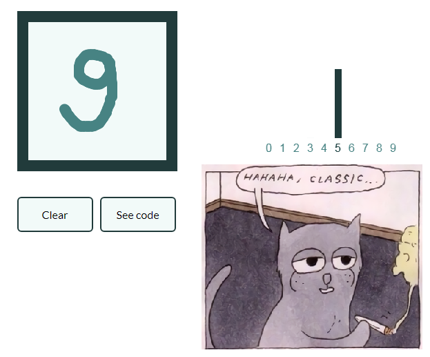
And here you can play with trained models

Installation

Download the distribution kit from the official site and install the Julia interpreter ( REPL ) on your computer.

For the package manager to work correctly, users of Windows 7 / Windows Server 2012 must also install:

TLS easy_fix For details, see Discourse thread .
Windows Management Framework 3.0 or later .

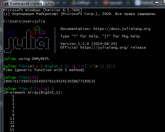
The process of working in REPL looks something like this:

True datasayantists and machine-lingologists prefer Jupyter . Here you can look about the installation, as well as find interactive lessons for independent study with assignments in Russian (links to original tutorials and a guide to the language there).

Here you can see how to work with the Jupyter Notebook.

If installation problems

Connection cannot be established - check your access rights (do you have restrictions on writing to folders on C: \, log in as admin or start Julia in administrator mode), if using a proxy, make sure that it is configured not only for the browser
Some packages do not like Cyrillic in the file path, so because of the username in Russian I had a lot of problems

If the Interact package does not display results, you may have installed WebIO incorrectly, which can be fixed

#]add WebIO using WebIO jup = WebIO.find_jupyter_cmd() WebIO.install_jupyter_nbextension( jup )

For some packages to work correctly on Windows, the paths to Julia and Jupyter must be entered in environment variables.

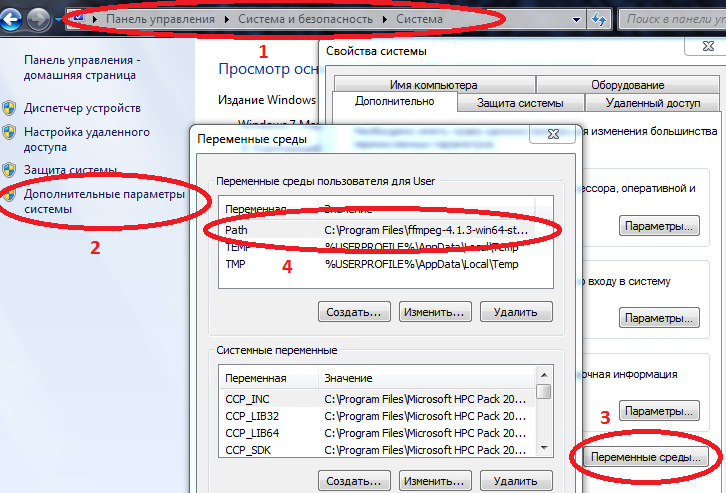
Computer / System properties / Advanced system parameters / Environment variables / Path (Create if not) and add the path to julia.exe there

Example C: \ Users \ User \ AppData \ Local \ Julia-1.2.0 \ bin

if Path already has values, then separate them with a semicolon.

Now if you drive julia

into the command console ( cmd ), the interpreter will start.

Having installed everything you need, you can proceed to download the packages you need today. Enter commands in REPL or Jupyter

The code

 using Pkg pkgs = ["Plots", "TextParse", "CSV", "DataFrames", "ImageMagick", "Images", "Interact", "Flux"] for p in pkgs Pkg.add(p) end for p in pkgs Pkg.build(p) end

After learning the basics of the language (working with arrays, creating functions, downloading packages, plotting graphs), you can proceed to the subsequent material.

Data loading and processing

Collecting and organizing data is a separate art. Regarding Julia, the network has a lot of outdated material, but for starters you can try the above tutorial , and for a more thorough study, read the book Data Science with Julia (in the public domain)

And today, perhaps, we ’ll work with already prepared data: a dataset from a huge number of photographs of fruits from various angles - who wanted a fruit fresh?

Actually this is the task - we will teach the neural network to distinguish apples from bananas!

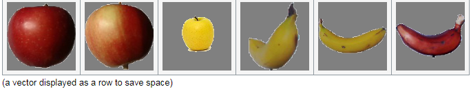
First things first, upload some test images:

 using Images fnames = [ "data/10_100.jpg", "data/107_100.jpg", "data/yellow_apple_2.jpg", "data/8_100.jpg", "data/104_100.jpg", "data/3_100.jpg" ] #   fruits = [load(fname) for fname in fnames] hcat(fruits...) #

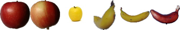
How do the objects in the pictures differ from each other? Firstly, by form, secondly by color, and then by textures and other attributes. Image analysis is an interesting topic in itself, and classification can be made not only by neurons, but also, say, by wavelets . We will start with the simplest sign - color.

As you know, images are stored in computer memory in the form of arrays, in our case these are matrices, each cell of which contains three numbers, indicating the amounts of red, green and blue colors in each pixel of the image. Let's see the average amount of each color in these images:

 using Statistics: mean M1 = [ mean(float.(c.(img))) for c = [red,green,blue], img = fruits ] 3×6 Array{Float32,2}: 0.570278 0.652852 0.977111 0.835252 0.903998 0.842564 0.338118 0.468729 0.950773 0.806882 0.880692 0.755442 0.322406 0.379424 0.835212 0.707626 0.799643 0.761916

We carefully look at the first line - doesn’t it bother you? A yellow apple and bananas are redder than apples of the Breburn variety! How so ?! Come on, make up sour mines, maybe the schoolchildren are reading this tutorial, or younger students from the Ballet and Tractor Institute. Therefore, we will try to avoid omissions. The fact is that the background of each picture is white, and in RGB notation it is represented by the values (1,1,1). And since there are 6 more backgrounds on the 3 dash images, plus the coloring of the bananas and the yellow apple also contains red, it turns out that the first two pictures lose in red. For clarity, we split the images into basic colors:

 function tweaking(img) R = colorview( RGB, red.(img),zeroarray,zeroarray ) G = colorview( RGB, zeroarray,green.(img),zeroarray ) B = colorview( RGB, zeroarray,zeroarray, blue.(img) ) [R; G; B] end tweaking( hcat(fruits...) )

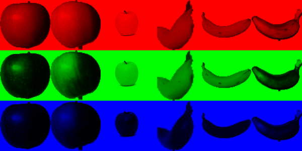
Have you ever heard the cryptic word "basis?" So, we can say that these images are laid out in an RGB basis. The blacker - the less a certain color, and as we expected, the background with its richness makes the calculation of averages noisy. Delete it.

 function remove_background(img) mtrx = copy( channelview(img) ) for i = 1:size(mtrx, 2), j = 1:size(mtrx, 3) if reduce(&, mtrx[:,i,j] .> [0.8, 0.8, 0.8]) #   -  mtrx[:,i,j] .= [0.5, 0.5, 0.5] end end colorview(RGB, mtrx) end greyfruits = remove_background.(fruits)

 M3 = [ mean(float.(c.(img))) for c = [red,green,blue], img = greyfruits ] 3×6 Array{Float32,2}: 0.451008 0.532696 0.578967 0.527727 0.52849 0.500276 0.218805 0.348609 0.552679 0.499192 0.505136 0.412946 0.203528 0.260142 0.439354 0.400631 0.424784 0.419291

The difference in the area occupied by each object is still affecting, but in general, it can be concluded that bananas are greener ( and blue ) apples. This will be the evaluation criterion, that is - a sign. Now let's take a look at the rest of the pictures:

 pth = "C:\\Users\\User\\Desktop\\Banana" # Apple Braeburn fnames = readdir(pth)[1:300] 300-element Array{String,1}: "0_100.jpg" "104_100.jpg" "107_100.jpg" "10_100.jpg" "112_100.jpg" "117_100.jpg" "118_100.jpg" "119_100.jpg" ...

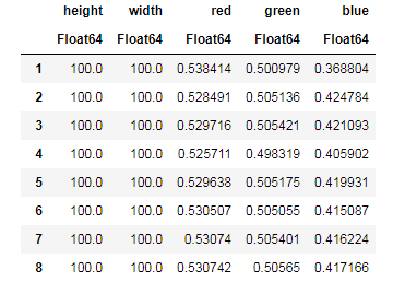
For each image we level out the contribution of the background, we find the average amount of each color, simultaneously remembering the size of the images ...

 dataz = [] for fname in fnames img_i = load("$pth\\$fname") gbimg = remove_background(img_i) colorz = [ mean(c.(gbimg)) for c = [red,green,blue] ] inform = [size(gbimg, 1) size(gbimg, 2) colorz' ] push!(dataz, inform) end dataz

... and then you can arrange our data in structures convenient for work - data frames:

 using DataFrames, CSV banans = DataFrame( vcat(dataz...), [:height, :width, :red, :green, :blue] ) CSV.write("data/bananas.csv", banans) #

 apples = CSV.read("data/Apple_Braeburn.csv") #    banans = CSV.read("data/bananas.csv")

 Desc = describe(apples, :all) #

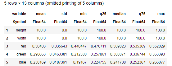
Try to comprehend the data provided by the describe()

function and compare with a similar table for bananas. Well, what kind of data analysis can be without graphs?

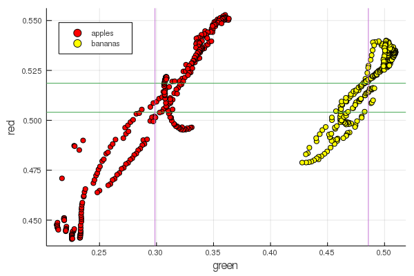
 function plot2features(clr) x_apples = apples[:, :green] x_banans = banans[:, :green] y_apples = apples[:, clr] y_banans = banans[:, clr] scatter(x_apples, y_apples, lab = "apples", colour = :red) scatter!(x_banans, y_banans, lab = "bananas", legend = :topleft, colour = :yellow) hline!([mean(y_apples), mean(y_banans) ], lab = "" ) vline!([mean(x_apples), mean(x_banans) ], lab = "" ) xaxis!("green") yaxis!("$clr") end plot2features(:red)

 plot2features(:blue)

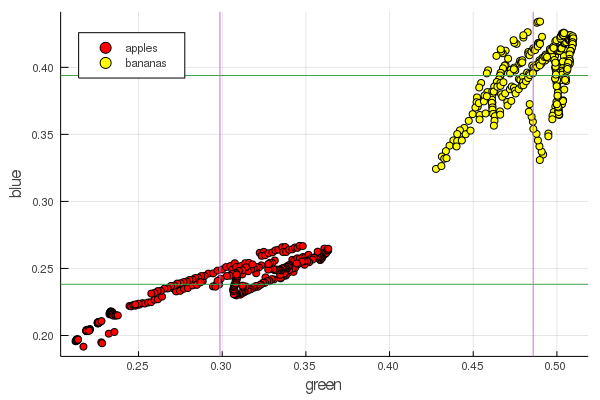
Mid-banana red is very close in value to mid-apple. But on the second chart, the isolation of fruits is immediately more clearly traced by two color characteristics at once. Separations can be improved by correct renormalization, for example, our green values change from 0.2 to 0.55, and if you perform the conversion

x_{i}^{'} = f r a c x_{i} - m i n (x) m a x (x) - m i n (x)

$x_i '= \ frac {x_i - \ min (x)} {\ max (x) - \ min (x)}$

then we get the data rescaled by [0,1], which will increase the gap between these ~~heaps~~ clusters of points.

Perceptron

The classification task consists in setting a model and selecting parameters for which various data will uniquely receive an assessment of their belonging to a particular class. Simply put, we need to introduce a certain function and set its parameters so that it separates our apples from bananas.

The most famous and popular model for these purposes is the McCulloch-Pitts artificial neuron, developed in the early 1940s. Subsequently, Frank Rosenblatt proposed a trained neural network - the perceptron. It is not difficult to find comprehensive explanations about neural networks, including on this resource (for example, Neural networks for beginners , Use of neural networks in image recognition , Neural networks, fundamental principles of operation, diversity and topology )

Selecting the sigmoid as the activation function and setting the outputs of the classified objects (fruits) in accordance with its outputs

s i g m a (x; w, b) := f r a c 1 1 + e x p (- w x + b)

$\ sigma (x; w, b): = \ frac {1} {1 + \ exp (-wx + b)}$

x = m a t h r m d a t a

$x = \ mathrm {data}$

s i g m a (x; w, b) a p p r o x 0 i m p l i e s m a t h r m a p p l e

$\ sigma (x; w, b) \ approx 0 \ implies \ mathrm {apple}$

s i g m a (x; w, b) a p p r o x 1 i m p l i e s m a t h r m b a n a n a

$\ sigma (x; w, b) \ approx 1 \ implies \ mathrm {banana}$

select such parameters $W$ and $b$ so that the output values of the sigmoid for the received data correspond to the above notation

 using Interact sigmo(x,w,b) = 1 / (1 + exp(-w*x+b)) r_apples, g_apples, b_apples = apples[:, :red], apples[:, :green], apples[:, :blue] r_banans, g_banans, b_banans = banans[:, :red], banans[:, :green], banans[:, :blue]; @manipulate for w in 10:1:60, b in -5:1:25 plot(x->sigmo(x,w,b), 0, 1, label="Model", legend = :topleft, lw=3) scatter!(g_apples[1:5], zeros(10), label="Apple", colour = :red) scatter!(g_banans[1:5], ones(10), label="Banana", colour = :yellow) end

 foon(x) = sigmo(x,60,24) plot(foon, 0, 1, label="Model", legend = :topleft, lw=3) scatter!(foon, g_apples, label="Apple", colour = :red) scatter!(foon, g_banans, label="Banana", colour = :yellow) xaxis!("green")

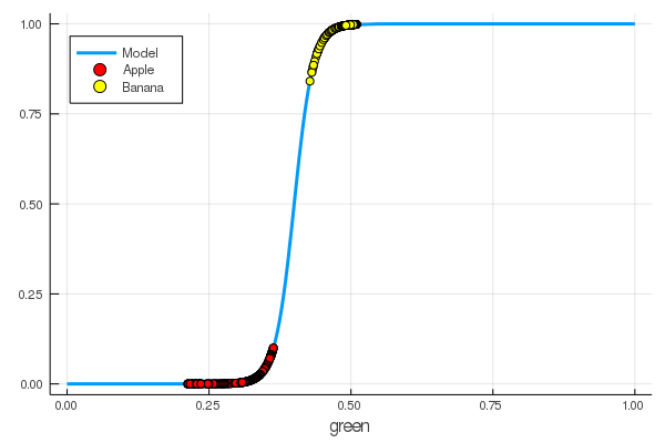
We manually taught a neuron to distinguish apples from bananas by the amount of green!

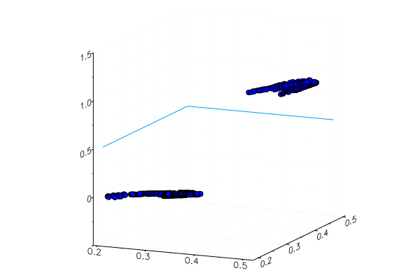
Naturally, the desire to automate this process. We introduce the loss function

L (w, b) = (0 - σ (x_{1}, w, b))^{2} + (1 - σ (x_{2}, w, b))^{2}

$L (w, b) = (0 - σ (x_1, w, b)) ^ 2 + (1 - σ (x_2, w, b)) ^ 2$

Now the learning process will consist in minimizing this function:

The code

 apples_mean_green = mean(g_apples) banans_mean_green = mean(g_banans) L(w, b) = (0 - sigmo(apples_mean_green,w,b))^2 + (1 - sigmo(banans_mean_green,w,b))^2 w_range = 10:0.5:30 b_range = 0:0.5:20 L_values = [L(w,b) for b in b_range, w in w_range] @manipulate for w in w_range, b in b_range p1 = surface(w_range, b_range, L_values, xlabel="b", ylabel="w", cam=(80,40), cbar=false, leg=false) scatter!(p1, [w], [b], [L(w,b)+1e-2], markersize=5, color = :blue) p2 = plot(x->sigmo(x,w,b), 0, 1, label="Model", legend = :topleft, lw=3) scatter!(p2, [apples_mean_green], [0.0], label="Apple", markersize=10) scatter!(p2, [banans_mean_green], [1.0], label="Banana", markersize=10, xlim=(0,1), ylim=(0,1)) plot(p1, p2, layout=(2,1)) end

Earlier we studied packages for Julia that allow solving optimization problems by various methods. Fortunately, the essentials are already in the Flux environment!

Flux

 using Flux

First, we present the data for training in a digestible form:

 Y = [zeros(length(g_apples)); ones(length(g_banans)) ] |> permutedims X = [g_apples; g_banans] |> permutedims; #   -   # dataz = repeated((X, Y), 20)

Next in order:

We create a training dataset by combining the input data with the correct answers regarding the classification of these data
We set the parameters W and b by matrices of random values (there is one sign at the input and one at the output, so matrices are 1 x 1 in size)
As a model, we set a dense layer - a perceptron with a sigmoidal activation function
We set the loss function - the sum of the squared differences (you can still use the more popular Flux.crossentropy()

)
As an optimization method, we choose gradient descent . It takes a parameter - descent speed
We set an evaluation function that will round the values of the model outputs and compare them with the correct answers.
And print the parameters of our untrained model

 dataz = [(X, Y)] W = param(rand(1)) b = param(rand(1)) model = Dense(W, b, σ) loss(x, y) = mse(model(x), y) opt = Descent(0.1) accuracy(x, y) = mean( round.(model(x)) .== y ) params(model) Params([[0.3372841444115968] (tracked), [0.8430399003786011] (tracked)])

Let's see what the output of the loss function is for our data.

 loss(X, Y) #  ,   0.310845210182773 (tracked)

And check the results of the evaluation function

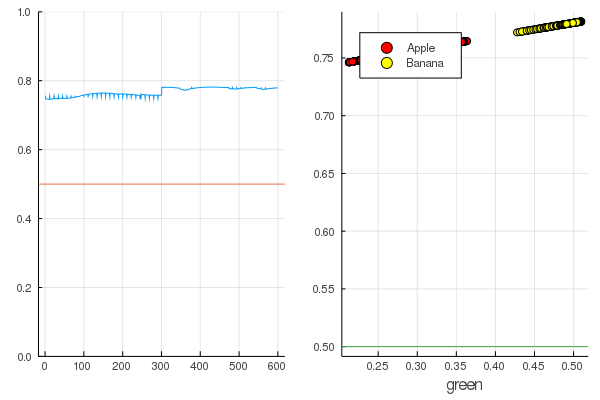
 accuracy(X, Y) 0.5

The result is quite natural - the outputs are distributed quite uniformly and half of the data is correctly classified:

The code

 modeldataz(x) = x |> model |> data |> permutedims # modeldataz(x) = permutedims(data(model(x)))

 modelX = modeldataz(X) modelapples = modeldataz(g_apples') modelbanans = modeldataz(g_banans') plot(modelX, legend = false) hline!([0.5]) p1 = yaxis!((0,1)) curv = [-1:0.01:1;]' |> modeldataz plot( [-1:0.01:1;], curv, label="Model", legend = :topleft, lw=3) scatter!(g_apples, modelapples, label="Apple", colour = :red) scatter!(g_banans, modelbanans, label="Banana",colour = :yellow) hline!([0.5], lab = "", legend = :topleft) p2 = xaxis!("green") plot(p1, p2)

Let's get started: it's pretty simple. You just need to shout at the neural network: “Train!”, While indicating what to train on and what to minimize, and she will complete one training session. Therefore, we will force her to wean everything as it should, but only without fanaticism, so that there is no retraining

 for i in 1:7000 train!(loss, params(model), dataz, opt) end model.W, model.b ([9.578663260720564] (tracked), [-3.7540362587506464] (tracked))

Losses have become much less:

 loss(X, Y) 0.09152783090457564 (tracked)

A rating is better:

 accuracy(X, Y) 1.0

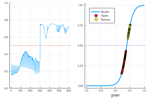
The data is divided, and further training will make the model function more vertical. Check the trained model on the very first set of fruits:

 function classifier(img) gbimg = remove_background(img) greenmean = [ mean(float.(c.(gbimg))) for c = [red,green,blue] ] answ = data( model( [ greenmean[2] ]' ) )[1] fr = answ > 0.5 ? "Banana" : "Apple" "$fr $(round(200abs(0.5-answ)))%" end hcat(fruits...)

 classifier.(fruits) 6-element Array{String,1}: "Apple 68.0%" "Apple 20.0%" "Banana 65.0%" "Banana 47.0%" "Banana 49.0%" "Banana 10.0%"

A specially planted yellow apple, of course, was not recognized correctly, and a red banana barely entered its category. But the neuron gets only one number from the picture - the average amount of green. You can add one more sign, say, the amount of blue, which will make the model a little more adaptable.

Or you can use not the RGB representation, but HSV (hue, saturation, value), in which the hue channel will contain information about the color of the image.

The whole relish of neural networks is that they themselves can distinguish features that are sometimes not very obvious (color correlation, their distribution, outlines and curves ...), but you can help them with the help of special heuristics and techniques, which turns work with neural networks into real art.

So that the leadership does not grow too much ~~and do a series of articles too lazy~~ Let us also give an example of the classification of pictures with handwritten numbers, and the interested reader will himself generalize the knowledge gained into images with fruits and create his own neural network, capable of, say, marking objects in still lifes!

Mnist

 using Images using Flux, Flux.Data.MNIST, Statistics using Flux: onehotbatch, onecold, crossentropy, throttle using Base.Iterators: repeated # using CuArrays # Classify MNIST digits with a simple multi-layer-perceptron imgs = MNIST.images() # Stack images into one large batch X = hcat(float.(reshape.(imgs, :))...); hcat(imgs[1:10]...)

An example is interesting in that there are already ten exits. So-called One-hot vectors come in handy here.

 labels = MNIST.labels() # One-hot-encode the labels Y = onehotbatch(labels, 0:9)

 10×60000 Flux.OneHotMatrix{Array{Flux.OneHotVector,1}}: 0 1 0 0 0 0 0 0 0 0 0 0 0 … 0 0 0 0 0 0 0 0 0 0 0 0 0 0 0 1 0 0 1 0 1 0 0 0 0 0 0 0 0 0 0 1 0 0 0 0 0 0 0 0 0 0 1 0 0 0 0 0 0 0 0 0 0 1 0 0 0 0 0 0 0 0 0 0 0 0 0 0 0 1 0 0 1 0 1 0 0 0 0 0 0 0 0 1 0 0 0 0 0 1 0 0 0 0 0 0 1 0 0 0 0 0 0 0 0 0 0 0 0 0 0 0 1 0 0 0 0 0 0 0 0 0 0 1 0 … 0 0 0 0 0 1 0 0 0 1 0 0 0 0 0 0 0 0 0 0 0 0 0 0 0 0 0 0 0 0 0 0 0 0 0 1 0 0 0 0 0 0 0 0 0 0 0 0 0 0 1 0 0 0 0 0 0 0 0 0 0 0 0 0 0 0 0 0 0 0 0 0 0 0 0 0 1 0 0 0 0 0 1 0 0 0 1 0 0 0 0 1 0 0 0 0 0 0 0 0 0 0 1 0 1 0 0 0 0 0 0 0

We define a chain of neurons as a model, the cross entropy will be the loss function, and Adam as the optimization method:

 m = Chain( Dense(28^2, 32, relu), Dense(32, 10), softmax) loss(x, y) = crossentropy(m(x), y) accuracy(x, y) = mean(onecold(m(x)) .== onecold(y)) dataset = repeated((X, Y), 20) evalcb = () -> @show(loss(X, Y)) opt = ADAM()

Train in a sparing mode, but printing out losses every 10 seconds:

 for i = 1:10 Flux.train!(loss, params(m), dataset, opt, cb = throttle(evalcb, 10)) end #   ...

 accuracy(X, Y) 0.64545

And check on the data not used in training

 # Test set accuracy tX = hcat(float.(reshape.(MNIST.images(:test), :))...) tY = onehotbatch(MNIST.labels(:test), 0:9) accuracy(tX, tY) 0.6488

Neural networks on Julia is simple and very exciting! Even if there is no need to look for connections between your field of activity and machine learning, you should at least feel this curiosity, which is shouted from all angles, and there will be no shortage of tools!

All moderate CPU heat!

Julia and Neural Networks: Flux

Installation

Data loading and processing

Perceptron

Flux

Mnist

More articles: