
Hello, Habr! We continue to publish reviews of scientific articles from members of the Open Data Science community from the channel #article_essense. If you want to receive them before everyone else - join the community !
Articles for today:
- Layer rotation: a surprisingly powerful indicator of generalization in deep networks? (Université catholique de Louvain, Belgium, 2018)
- Parameter-Efficient Transfer Learning for NLP (Google Research, Jagiellonian University, 2019)
- RoBERTa: A Robustly Optimized BERT Pretraining Approach (University of Washington, Facebook AI, 2019)
- EfficientNet: Rethinking Model Scaling for Convolutional Neural Networks (Google Research, 2019)
- How the Brain Transitions from Conscious to Subliminal Perception (USA, Argentina, Spain, 2019)
- Large Memory Layers with Product Keys (Facebook AI Research, 2019)
- Are We Really Making Much Progress? A Worrying Analysis of Recent Neural Recommendation Approaches (Politecnico di Milano, University of Klagenfurt, 2019)
- Omni-Scale Feature Learning for Person Re-Identification (University of Surrey, Queen Mary University, Samsung AI, 2019)
- Neural reparameterization improves structural optimization (Google Research, 2019)
1. Layer rotation: a surprisingly powerful indicator of generalization in deep networks?
Authors: Simon Carbonnelle, Christophe De Vleeschouwer (Université catholique de Louvain, Belgium, 2018)
→ Original article
Review author: Svyatoslav Skoblov (in slack error_derivative)

In this article, the authors drew attention to a rather simple observation: cosine distance between the layer weights during initialization and after training (the process of increasing the distance during training is called layer rotation). Gentlemen say that in most experiments, networks that have reached a distance of 1 in all layers stably outperform other configurations. The paper also presents the Layca algorithm (Layer-level Controlled Amount of weight rotation), which allows using this layer-wise learning rate to control this same layer rotation. In fact, it differs from the usual SGD algorithm by the presence of orthogonal projection and normalization. A detailed listing of the algorithm along with the training scheme can be found in the article.
The main idea that the authors deduce is: the larger the layer rotations, the better the generalization performance . Most of the article is a record of experiments where various training scenarios were studied: MNIST, CIFAR-10 / CIFAR-100, tiny ImageNet with different architectures were used, from a single-layer network to the ResNet family.
A series of experiments was broken into several stages:
- Vanilla SGD It turned out that, on the whole, the behavior of the scales coincides with the hypothesis (large changes in the distance corresponded to the best metric values), however, problems were noticed: layer rotation stopped long before the desired values; instability in changing distance was also noticed.
- SGD + weight decay Decreasing the weight norm greatly improved the training picture: most layers reached the maximum distance, and the test performance is similar to the proposed Layca. The undoubted advantage of the author’s method is the absence of an additional hyperparameter.
- LR warmups It turned out that warmup helps SGD overcome the problem of unstable layer rotation, however, it has no effect on Layca.
- Adaptive Gradient Methods In addition to the well-known truth (that using these methods it is harder to achieve the level of generalization that SGD + weight decay can give), it turned out that the effects of layer rotation are very different: the first increase rotation in the last layers, while SGD in the initial layers . The authors hint that this may be the meanness of adaptive methods. And they suggest using Layca in conjunction with them (improving the ability to generalize in adaptive methods and speeding up training in SGD).
The article concludes with an attempt to interpret the phenomenon. To do this, the authors trained a network with 1 hidden layer on a stripped-down version of MNIST, after which they visualized random neurons, reaching a quite logical conclusion: a large degree of layer rotation corresponds to a lesser effect of initialization and a better study of features, which contributes to improved generalization.
The code of the implemented algorithm (tf / keras) and the code for reproducing experiments are uploaded .
2. Parameter-Efficient Transfer Learning for NLP
Authors: Neil Houlsby, Andrei Giurgiu, Stanislaw Jastrzebski, Bruna Morrone, Quentin de Laroussilhe, Andrea Gesmundo, Mona Attariyan, Sylvain Gelly (Google Research, Jagiellonian University, 2019)
→ Original article
Review author: Alexey Karnachev (in slack zhirzemli)
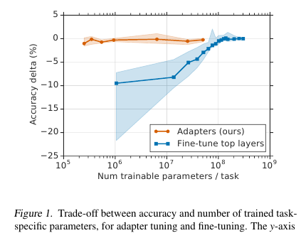
Here gentlemen offer a simple but effective fine-tuning technique for NLP models (in this case, BERT). The idea is to embed learning layers (adapters) directly into the network. Each such layer is a network with a bottleneck, which adapts the hidden states of the original model to a specific down-stream task. The weights of the original model, in turn, remain frozen.
Motivation
In the conditions of streaming-training (or near-online training), where there are many down-stream tasks, I don’t really want to file the whole model. Firstly, for a long time, and secondly, it is difficult, and thirdly, even if it is tight, the model needs to be somehow stored: to dump or to keep in memory. And we will no longer be able to reuse this model for the following task: each time we have to tune up a new one. As a result, we can try to adapt the hidden network conditions to the current problem. Moreover, the original model remains untouched, and the adapters themselves are much more capacious than the main model (~ 4% of the total number of parameters)
Implementation
The problem is solved in an incredibly simple way: we add 2 adapters to each layer of the model. Before layer normalization in transformer-based models, skip-connection occurs: the transformed input (current hidden state) is added to the original input.
There are 2 such sections in each transformer layer. One is after multi-head attention, the second is after feed forward. Thus, the hidden states of these sections are additionally passed through the Adapter: a shallow network with a 1-bottleneck hidden layer and with output the same dimension as input. Nonlinearity is applied to the bottleneck state, and Input (skip-connection) is added to the output. It turns out that the total number of trained parameters is: 2md + m + d, where d is the dimension of the hidden state of the original model, m is the size of the bottleneck adapter layer. It turns out that for the BERT-base model (12 layers, 110M parameters) and for the adapter-bottlneck size of 128, we get 4.3% of the total number of parameters
results
Comparison was made with full model tuning. For all tasks, this approach showed a minor loss in metrics (on average less than 1 point), with the number of trained weights - 3% of the total. I will not list the tasks themselves, there are many of them, there is a tablet in the article.
Fine tuning
In this model, only the Adapter part is tuned (+ the classifier at the output itself). For adapter scales, they propose to do near-identity initialization. Thus, an untrained model will not change the hidden network states in any way, and this will make it possible to decide which states to adapt for the task and which ones to leave unchanged during the model’s training.
Learning rate recommend taking more than with standard BERT finetuning. Personally, on my task, 1e-04 lr worked well. In addition, (already personally my observation) in the process of tuning the model almost always explodes gradients, so you need to remember to do clipping. Optimizer - Adam with warmup 10%
The code
The code in their article is attached. Implementation on Tensorflow .
For Torch, the author of the review forked pytorch-transformers and added an Adapter layer (at the beginning of the README.md file there is a small launch manual)
3. RoBERTa: A Robustly Optimized BERT Pretraining Approach
Authors: Yinhan Liu, Myle Ott, Naman Goyal, Jingfei Du, Mandar Joshi, Danqi Chen, Omer Levy, Mike Lewis, Luke Zettlemoyer, Veselin Stoyanov (University of Washington, Facebook AI, 2019)
→ Original article
Review author: Artem Rodichev (in slack fuckai)
Dramatically raised the quality of BERT models, the first place on the GLUE leaderboard and SOTA on many NLP tasks. They suggested a number of ways to train the BERT model as best as possible without any change to the model architecture itself.
Key differences with the original BERT:
- Increased train building 10 times, from 16 GB of raw text to 160 GB
- Made dynamic masking for each sample
- Removed the use of next sentence prediction loss
- Increased the size of the mini-batch from 256 samples to 8k
- Improved BPE encoding by transferring the database from Unicode to bytes.
The best final model was trained on 1024 Nvidia V100 cards (128 DGX-1 servers) for 5 days.
The essence of the approach:
Data. In addition to the Wiki corps and BookCorpus (16GB in total), which taught the original BERT, they added 3 more larger corps, all in English:
- SS-News 63 million news in 2.5 years on 76GB
- OpenWebText is the framework on which OpenAI was taught the GPT2 model. These are crawled articles to which links were given in posts on a reddit with at least three updates. 38GB data
- Stories - 31GB CommonCrawl Story Case
Dynamic masking. In the original BERT, 15% of tokens are masked in each sample and these tokens are predicted using the unmasked part of the sequence. A mask is generated for each sample once during preprocessing and does not change. At the same time, the same sample in the train can occur several times, depending on the number of eras in the body. The idea of dynamic masking is to create a new mask for the sequence each time, rather than using a fixed one in preprocessing.
Next Sentence Prediction objective. Let's just cut this objektiv and see if it got worse? Has it become better or has also remained - on SQuAD, MNLI, SST and RACE tasks.
Increase the size of the mini-batch. In many places, in particular in Machine Translation, it was shown that the larger the mini-batch, the better the final results of the train. They showed that if you increase the minibatch from 256 samples, as in the original BERT, to 2k, and then to 8k, then perplexity on validation drops, and the metrics on MNLI and SST-2 grow.
BPE The BPE from the original BERT implementation uses Unicode characters as the base for subword units. This leads to the fact that on large and diverse cases a significant part of the dictionary will be occupied by individual Unicode characters. OpenAI back in GPT2 suggested using not Unicode characters, but bytes as the base for subwords. If we use a 50k BPE dictionary, then we will not have unknown tokens. Compared to the original BERT, the model size increased by 15M parameters for the base model and by 20M for large, that is, 5-10% more.
Results:
BERT-large and XLNet-large are used as models for comparison. RoBERTa itself is the same in parameters as BERT-large. As a result, they won first place on the GLUE benchmark. We used single-task file tuning, unlike many other approaches from the GLUE benchmark top that do multi-task file tuning. On the girls in GLUE, single model results are compared, they got SOTA on all 9 tasks. On the test set they compare the ensemble of models, SOTA for 4 of 9 tasks and the final glue speed. On two versions of SQuAD on the SOTA dev network, on the test set at XLNet level. Moreover, unlike XLNet, they don’t get caught on additional QA packages before solving SQuAD.

SOTA on RACE task in which a piece of text is given, a question on this text and 4 answer options where you need to choose the right one. To solve this task, they concatenate the text, question and answer, run through BERT, get a representation from the CLF token, serve on one fully connected layer and predict whether the answer is correct. This is done 4 times - for each of the answer options.
We posted the code and pretrain of the RoBERTa model in fairseq turnip . You can use it, everything looks neat and simple.
4. EfficientNet: Rethinking Model Scaling for Convolutional Neural Networks
Authors: Mingxing Tan, Quoc V. Le (Google Research, 2019)
→ Original article
Review author: Alexander Denisenko (in slack Alexander Denisenko)

They study the scaling (scaling) of models and balancing between themselves the depth and width (number of channels) of the network, as well as the resolution of images in the grid. They offer a new scaling method that uniformly scales depth / width / resolution. Show its effectiveness on MobileNet and ResNet.
They also use Neural Architecture Search to create a new mesh and scale it, thereby obtaining a class of new models - EfficientNets. They are better and much more economical than previous grids. On ImageNet, EfficientNet-B7 achieves state-of-the-art 84.4% top-1 and 97.1% top-5 accuracy, while being 8.4 times less and 6.1 times faster on inference than the current best-in-class ConvNet. It transfers well to other datasets - they got SOTA on 5 of the 8 most popular datasets.
Compound model scaling
Scaling is when operations performed inside the grid are fixed and only the depth (the number of repetitions of the same modules) d, width (number of channels in convolution) w and resolution r are changed. In the pager, scaling is formulated as an optimization problem - we want maximum Accuracy (Net (d, w, r)) despite the fact that we do not crawl out of bounds in memory and in FLOPS.
We conducted experiments and made sure that it really helps also to scale in depth and resolution when scaling in width. With the same FLOPS, we achieve a significantly better result on ImageNet (see the picture above). In general, this is reasonable, because it seems that when increasing the resolution of the network image, more layers are needed in depth to increase the receptive field and more channels in order to capture all the patterns in the image with a higher resolution.
The essence of compound scaling: we take the compound coefficient phi, which uniformly scales d, w and r with this coefficient: Where - constants obtained from a small grid of sirch on the initial grid. - coefficient characterizing the amount of available computing resources.
Efficient net
To create the grid, we used Multi-objective neural architecture search, optimized Accuracy and FLOPS with the parameter responsible for the trade-off between them. Such a search gave EfficientNet-B0. In short - Conv followed by several MBConv, at the end of Conv1x1, Pool, FC.
Then do the scaling in two steps:
- To begin, we fix , do grid search for search .
- Scale the grid using the formulas for d, w and r. Got EffiientNet-B1. Similarly, increasing , get EfficientNet-B2, ... B7.
Scaled for different ResNet and MobileNet, everywhere received significant improvements on ImageNet, compound scaling gave a significant increase compared to scaling in only one dimension. We also conducted experiments with EfficientNet on eight more popular datasets, everywhere we got SOTA or a result close to it with a significantly smaller number of parameters.
5. How the Brain Transitions from Conscious to Subliminal Perception
Authors of the article: Francesca Arese Lucini, Gino Del Ferraro, Mariano Sigman, Hernan A. Makse (USA, Argentina, Spain, 2019)
→ Original article
Review author: Svyatoslav Skoblov (in slack error_derivative)
This article is a continuation and rethinking of the work of Dehaene, S, Naccache, L, Cohen, L, Le Bihan, D, Mangin, JF, Poline, JB, & Rivie`re, D. Cerebral mechanisms of word masking and unconscious repetition priming , in which the authors tried to consider the modes of conscious and unconscious brain function.
Experiment:
Volunteers are shown pictures (4-letter words, or a blank screen, or scribbles). Each of them is shown for 30 ms, in general, the whole action lasts 5 minutes.
- In the "conscious" mode of the experiment, a blank screen alternates with words, which allows a person to consciously perceive the text.
- In the “unconscious” mode, words alternate with scribbles, which quite effectively prevented the perception of the text at a conscious level.
Data:
During this presentation, the brains of our primates were scanned using fMRI. In total, the researchers had 15 volunteers, each repeated the experiment 5 times, a total of 75 fMRI streams. It is worth noting that the voxel scan turned out to be quite large (very simplified: voxel is a 3D cube containing a fairly large number of cells) - 4x4x4mm.
Magic:
Let's call the node active voxel from our stream. Since the brain is a modular washcloth, we introduce two types of connections in it: external and internal (corresponding to the spatial arrangement of the nodes). Connections are assembled in an interesting way: we build a cross-correlation matrix between nodes and connect the nodes with a connection if the correlation is greater than some adaptive parameter lambda. This parameter affects the discharge of our network.
Parameter setting is carried out using the "filtering" procedure. If we sway our lambda a little, sharp transitions between the final dimensions of the network become noticeable (i.e., a sufficiently small change in the parameter corresponds to a large increment in size).
So: internal connections are activated by the lambda-1 value, which corresponds to the lambda value right before a sharp transition. External - lambda-2 value corresponding to the lambda value immediately after a sharp transition.
Magic 2:
k-core filtering. The k-core concept describes network connectivity and is formulated quite simply: the maximum subnet, all of whose nodes have at least k neighbors. Such a subnet can be obtained by iterative removal of nodes with less than k neighbors. Since the remaining nodes will lose neighbors, the process continues until there is nothing to delete. What remains is the k-core network.
Results:
Applying this artillery to our brains, you can see a number of very interesting features.
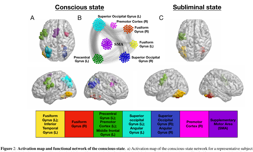
- The number of nodes in k-core with small / very large k is extremely large. But for medium k, on the contrary, it is not enough. In the picture, it looks like a U shape, namely, such a network configuration gives the greatest stability of the system (resistance to both local and global errors).
- and most important Nodes belonging to k-core with small k can be seen in almost any state of the network. But a k-core with very large k is characteristic only for those parts of the brain that are active in the unconscious state fusiform gyrus & left precentral gyrus . The same parts of the cortex are most active and in a conscious state.
To check the result, the authors created a million random networks based on real ones, doing random rewiring, while maintaining the original degree of the nodes (the same as the degree of the vertex in the graph). Real networks differed from random ones by much larger values of maximum k. At the same time, the U shape of the number of nodes in the clusters remained noticeable in random networks, which prompted the authors to the idea that it is the degree of the nodes that is responsible for this phenomenon.
Conclusions:
The authors, scratching their heads, reflect on the fact that the transition from the conscious to the unconscious in the brain occurs by weakening interactions in networks. Having scratched their heads on the other hand, they make the assumption that all external stimuli are processed unconsciously, and that consciousness is assigned only the role of a certain information regulator (hereinafter, researchers refer to other works, which, however, do not clarify the specific role of consciousness).
Moreover, based on the fact that the activation of networks in a conscious mode is quite diverse, it suggests itself that consciousness is not realized within a certain brain structure, but is an adaptive control response to unconscious stimuli and, therefore, each conscious impression -Is unique. Which, however, is not news and was known to the ancient Greeks as the qualia problem.
6. Large Memory Layers with Product Keys
Authors: Guillaume Lample, Alexandre Sablayrolles, Marc'Aurelio Ranzato, Ludovic Denoyer, Hervé Jégou (Facebook AI Research, 2019)
→ Original article
Review author: Maxim Lashkevich (in slack belerafon)

They tell how to make fast and differentiable key-value memory and where to shove it in already known architectures in order to get profit.
The memory is essentially a mixture of embedding and attention. There is a query vector q, memory has keys k and values v. We take q, multiply by all k, take the softmax from this, and we weight all the values from it and add up. This is what can be called the already famous memory architecture. The rest of the article says that there are two bottlenecks with a large amount of memory. If you take softmax from all the memory, then later you will have to back-drink it on learning, which is very painful. It is proposed to take only a few keys as close as possible to the q query and only take softmax from them (for example, top-10). Then you’ll only have to back up for the most relevant keys. This is like a well-known technique, too.
The second bottleneck is the calculation of the product of the query q by the keys k for the entire memory. It's long too, so the Product Keys trick is offered. The nuances are best viewed in the article, but in a nutshell they divide the query vector q into two parts, and all the keys are also cut in half. Performing the same operations to select the top 10 with these halves, it turns out that the search is performed instead of O (N) operations as in the "normal" memory implementation, but in total O (sqrt (N)).
The result is a large and fast and differentiable key-value memory. They offer to shove it in tasks where models underfit (where the dataset is such that the model cannot overfix). For example, they take BERT and train on a 28 billion word dataset. They show that it is better and faster to take a smaller capacity of the model itself, but expand it with such a memory. Namely: a 12-layer transformer with memory works 2 times faster than a 24-layer one with memory, and even perplexity with memory one point below.
They propose to put memory specifically in this architecture instead of a fully connected network (in the transformer it stands after self-attention layers). It is said that mathematically such a memory is essentially a fully-connected network with an incredibly large hidden layer. They also say that making memory queries is better in the style of multy-head attention. Those. instead of a single query, form several, select several value answers from them, summarize and spit it all out. So memory is used more intensively and more capaciously.
Well, in the article there are a lot of pictures and plates showing how much percent is used under what configurations, how much speed increases, where it is better to insert it into BERT. Nothing is written about other architectures.
7. Are We Really Making Much Progress? A Worrying Analysis of Recent Neural Recommendation Approaches
Authors of the article: Maurizio Ferrari Dacrema, Paolo Cremonesi, Dietmar Jannach (Politecnico di Milano, University of Klagenfurt, 2019)
→ Original article
Review author: Andrey Kuznetsov (in slack netcitizen)

The question of reproducibility of research results in the field of DL is raised with enviable regularity, however, in addition to reproducibility, even at large conferences there are often articles with omissions on the methodology.
Tasks
In this article, the authors tried to figure out how well everything is with the latest DL studies in the field of solving the applied problems of top-n recommendations. To do this, they took the DL recommendation algorithms of recent years with KDD, SIGIR, TheWebConf (WWW) and RecSys and tried to do the following things:
- Reproduce the results of the original articles
- Take the baseline of classic reko-algorithms and pull them for the corresponding datasets
- Compare the new algorithm with adequate baselines
results
- Only 7/18 (39%) were able to play
- In almost all of the reproduced articles, there were “subtleties” like the nonrandomness of the train / test partition, the strange calculation of metrics, etc., which often allow us to achieve the stated results.
- All but one of the algorithms (Variational Autoencoders for Collaborative Filtering (Mult-VAE) showed ± the same results) by a margin lost by the defunct KNN, SVD, PR.
conclusions
The popularity of DL, as a tool for solving problems in CVs, NLP does not give rest to recommender systems, but so far the results are not so encouraging.
8. Omni-Scale Feature Learning for Person Re-Identification
: Kaiyang Zhou, Yongxin Yang, Andrea Cavallaro, Tao Xiang (University of Surrey, Queen Mary University, Samsung AI, 2019)
→
: ( graviton)
Person Re-Identification, Face Recognition, , . (Kaiyang Zhou) deep-person-reid , (OSNet), Person Re-Identification. .
Person Re-Identification:

:
- conv1x1 deepwise conv3x3 conv3x3 (figure 3).
- , . ResNeXt , Inception (figure 4).
- “aggregation gate” . , Inception .

OSNet , .. , : ( , ) .
ReID OSNet ( 2 ) (Market: R1 93.6%, mAP 81.0% OSNet R1 87.0%, mAP 69.5% MobileNetV2) ResNet DenseNet (Market: R1 94.8%, mAP 84.9% OSNet R1 94.8%, mAP 86.0% ResNet).
: . OSNet “unsupervised domain adaptation” ( ).
ImageNet, MobileNetV2 , .
9. Neural reparameterization improves structural optimization
: Stephan Hoyer, Jascha Sohl-Dickstein, Sam Greydanus (Google Research, 2019)
→
: ( Arech)
/ - . , , , // / /, . "" , — , .
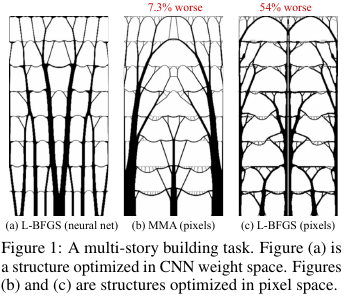
? : ( UNet), , , — (, , — ) . , , , . .
( ) , — ( 99 66 116 ). , .
Those. , ( ) ( ).