Looking for pneumonia in x-rays with Fast.ai

I came across an article on the blog of the School of Data company and decided to check what the Fast.ai library is capable of on the same dataset that is mentioned in the article. Here you will not find arguments about how important it is to timely and correctly diagnose pneumonia, whether radiologists will be needed in the conditions of technological development, whether the prediction of a neural network can be considered a medical diagnosis, etc. The main goal is to show that machine learning in modern libraries can be quite simple (literally requires a few lines of code) and gives excellent results. Let us remember the result from the article (precision = 0.84, recall = 0.96) and see what happens with us.



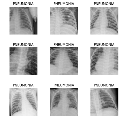
We take the data for training from here . The data are 5856 x-rays distributed in two classes - with or without signs of pneumonia. The task of the neural network is to give us a high-quality binary classifier of X-ray images to determine the signs of pneumonia.



We start by importing the libraries and some standard settings:

%reload_ext autoreload %autoreload 2 %matplotlib inline from fastai.vision import * from fastai.metrics import error_rate import os
      
      

        
        
        
      

    
        
        
        
      
      

        
        
        
      

    
     

Next, determine the batch size. When learning on the GPU, it is important to choose it in such a way that your memory is not full. If necessary, it can be halved.

 bs = 64
      
      

        
        
        
      

    
        
        
        
      
      

        
        
        
      

    
     

Important Update:

As rightly noted in the comments below, it is important to clearly monitor the data on which the model will be trained and on which we will test its effectiveness. We will train the model in the images in the train and val folders, and validate in the images in the test folder, similar to what was done here .



We determine the paths to our data

 path = Path('storage/chest_xray') path.ls()
      
      

        
        
        
      

    
        
        
        
      
      

        
        
        
      

    
     

and check that all the folders are in place (the val folder has been moved to train):

 Out: [PosixPath('storage/chest_xray/train'), PosixPath('storage/chest_xray/test')]
      
      

        
        
        
      

    
        
        
        
      
      

        
        
        
      

    
     

We are preparing our data for the “download” to the neural network. It is important to note that in Fast.ai there are several methods for matching the image label. The from_folder method tells us that labels should be taken from the name of the folder in which the image is located.



The size parameter means that we resize all images to a size of 299x299 (our algorithms work with square images). The get_transforms function gives us image augmentation to increase the amount of data for training (we leave the default settings here).

 np.random.seed(5) data = ImageDataBunch.from_folder(path, train = 'train', valid = 'test', size=299, bs=bs, ds_tfms=get_transforms()).normalize(imagenet_stats)
      
      

        
        
        
      

    
        
        
        
      
      

        
        
        
      

    
     

Let's look at the data:

 data.show_batch(rows=3, figsize=(6,6))
      
      

        
        
        
      

    
        
        
        
      
      

        
        
        
      

    
     

To check, we look at what classes we got and what quantitative distribution of images between train and validation:

 data.classes, data.c, len(data.train_ds), len(data.valid_ds)
      
      

        
        
        
      

    
        
        
        
      
      

        
        
        
      

    
     

 Out: (['NORMAL', 'PNEUMONIA'], 2, 5232, 624)
      
      

        
        
        
      

    
        
        
        
      
      

        
        
        
      

    
     

We define a training model based on the Resnet50 architecture:

 learn = cnn_learner(data, models.resnet50, metrics=error_rate)
      
      

        
        
        
      

    
        
        
        
      
      

        
        
        
      

    
     

and start learning in 8 eras based on One Cycle Policy :

 learn.fit_one_cycle(8)
      
      

        
        
        
      

    
        
        
        
      
      

        
        
        
      

    
     

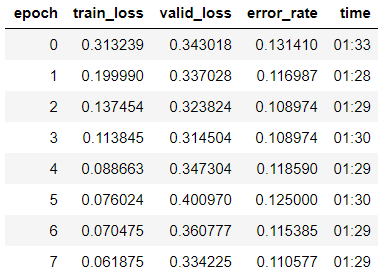
We see that we have already obtained an accuracy of 89% in the validation sample. We will write down the weights of our model for now and try to improve the result.

 learn.save('step-1-50')
      
      

        
        
        
      

    
        
        
        
      
      

        
        
        
      

    
     

“Defrost” the whole model, because before that, we trained the model only on the last group of layers, and the weights of the rest were taken from the model pre-trained on Imagenet and “frozen”:

 learn.unfreeze()
      
      

        
        
        
      

    
        
        
        
      
      

        
        
        
      

    
     

We are looking for the optimal learning rate to continue learning:

 learn.lr_find() learn.recorder.plot()
      
      

        
        
        
      

    
        
        
        
      
      

        
        
        
      

    
     

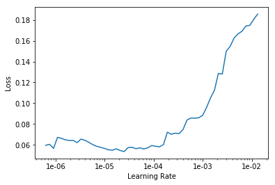
We start training for 10 eras with different learning rates for each group of layers.

 learn.fit_one_cycle(10, max_lr=slice(1e-6, 1e-4))
      
      

        
        
        
      

    
        
        
        
      
      

        
        
        
      

    
     

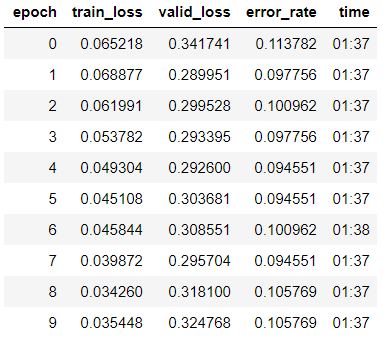
We see that the accuracy of our model slightly increased to 89.4% in the validation sample.



We write down the weights.

 learn.save('step-2-50')
      
      

        
        
        
      

    
        
        
        
      
      

        
        
        
      

    
     

Build Confusion Matrix:

 interp = ClassificationInterpretation.from_learner(learn) interp.plot_confusion_matrix()
      
      

        
        
        
      

    
        
        
        
      
      

        
        
        
      

    
     

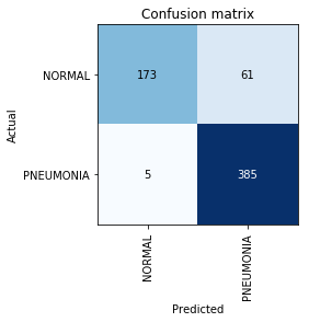
At this point, we recall that the accuracy parameter itself is not sufficient, especially for unbalanced classes. For example, if in real life pneumonia occurs only in 0.1% of those who undergo an X-ray examination, the system can simply give out the absence of pneumonia in all cases and its accuracy will be at the level of 99.9% with absolutely zero utility.



This is where Precision and Recall metrics come into play:

• TP - true positive prediction;
• TN - true negative prediction;
• FP - false positive prediction;
• FN - False Negative Prediction.

$$

$$Precision = TP / (TP + FP) = 385/446 = 0.863$$

$$

$$Recall = TP / (TP + FN) = 385/390 = $ 0.98$$

We see that our result is even slightly higher than the one mentioned in the article. In further work on the task, it is worth remembering that Recall is an extremely important parameter in medical problems, because False Negative errors are the most dangerous from the point of view of diagnostics (meaning that we can simply “overlook” a dangerous diagnosis).