The softest and most furry path in Machine Learning and Deep Neural Networks
Modern machine learning allows you to do incredible things. Neural networks work for the benefit of society: they find criminals, recognize threats, help diagnose diseases and make difficult decisions. Algorithms can surpass a person in creativity: they paint pictures, write songs and make masterpieces from ordinary pictures. And those who develop these algorithms are often presented as caricatured scientists.
Not everything is so scary! Anyone who is somewhat familiar with programming can build a neural network from basic models. And it’s not even necessary to learn Python, everything can be done in native JavaScript. It’s easy to get started and why machine learning is needed for front-end vendors , said Alexey Okhrimenko ( obenjiro ) at FrontendConf, and we transferred it to the text so that architecture names and useful links were at hand.
This story:
About the speaker: Alexei Okhrimenko works at Avito in the Frontend Architecture department, and in his free time conducts the Angular Moscow Meetup and releases the “Five Minute Angular”. Over a long career, he developed the design pattern MALEVICH, the PEG grammar parser SimplePEG. Alexey CSSComb maintainer regularly shares knowledge about new technologies at conferences and in his JS machine learning telegram channel .
Voice assistants, Siri, Google Assistant, Alice, are popular and often found in our lives. Many products have switched from conventional algorithmic data processing to machine learning. A striking example is Google Translate.

All the innovations and the coolest chips in smartphones are based on machine learning.

For example, Google NightSight uses machine learning. The cool photos that we see were not taken with lenses, sensors, or stabilization, but with machine learning. The machine finally beat people in DOTA2, which means that we have little chance of defeating artificial intelligence. Therefore, we must master machine learning as quickly as possible.
What is our daily programming routine, how do we usually write functions?
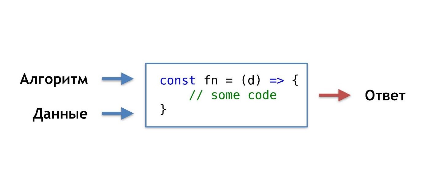
We take data and an algorithm that we ourselves invented or took from popular ready-made ones, combine, do a little magic and get a function that gives us the right answer in a given situation.
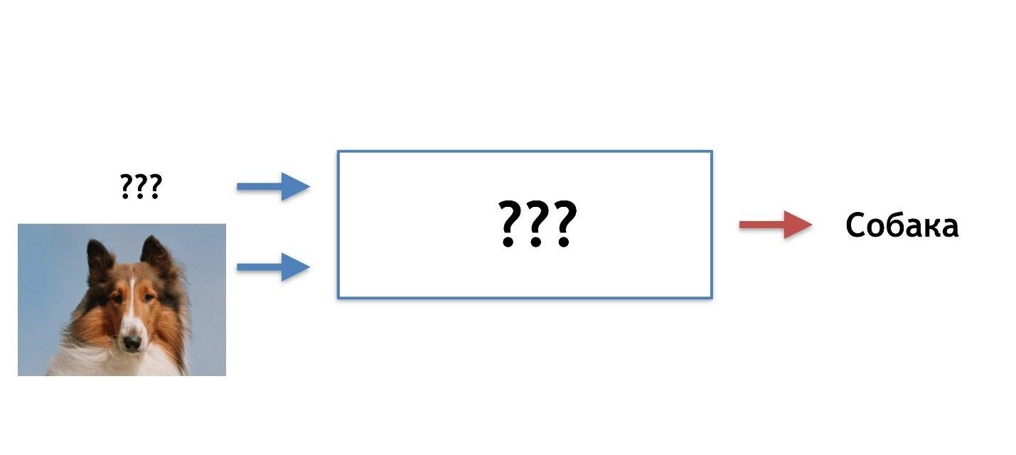
We are accustomed to this order of things, but there would be such an opportunity, without knowing the algorithm, but simply having the data and the answer, get the algorithm from them.

You can say: "I am a programmer, I can always write an algorithm."
Ok, but for example, what algorithm is needed here?

Suppose that the cat has sharp ears, and the dog’s ears are sluggish, small, like a pug.

Let's try to understand by ears who is who. But at some point, we find out that dogs can have sharp ears.
Our hypothesis is not good, we need other characteristics. Over time, we will learn more and more details, thereby demotivating ourselves more and more, and at some point we will want to quit this business altogether.
I imagine an ideal picture like this: in advance there is an answer (we know what kind of picture it is), there is data (we know that a cat is drawn), we want to get an algorithm that could feed data and get answers at the output.
There is a solution - this is machine learning, namely one of its parts - deep neural networks.
Machine learning is a huge area. It offers a gigantic amount of methods, and each one is good in its own way.
One of them is Deep Neural Networks. Deep learning has an undeniable advantage due to which it has become popular.
To understand this advantage, let's look at the classic classification problem using cats and dogs as an example.
There is data: pictures or photos. The first thing to do is embedding (embedding), that is, transform the data so that the machine is comfortable working with them. It’s inconvenient to work with pictures, the car needs something simpler.
First, align the pictures and remove the color. No matter what color the dog or cat is, it is important to determine the type of animal. Then we turn the pictures into arrays, where, for example, 0 is dark, 1 is light.

With this presentation of data, neural networks can already work.
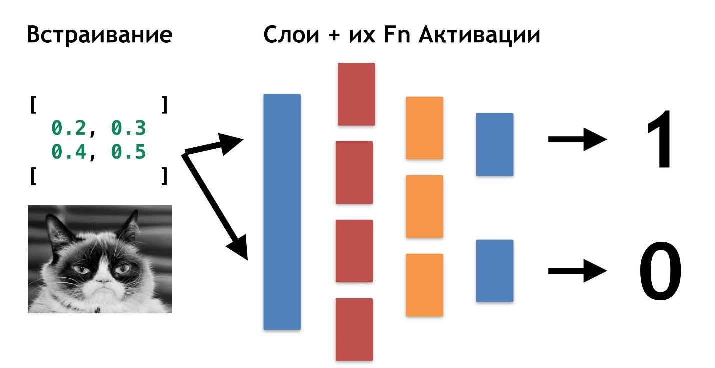
Let's create two more arrays and merge them into a certain “layer”. Next, we multiply each of the elements of the layer and the data array with each other using a simple matrix multiplication, and we direct the result into two activation functions (we will later analyze what these functions are). If the activation function receives a sufficient number of values, then it “activates” and produces the result:
This approach to coding a response is called One-Hot Encoding .

Already, several features of deep neural networks are noticeable:
It is not necessary to know what a cat is, what a dog is. It is enough to select the necessary numbers for an additional layer.
So far, the only thing that remains unclear is why these networks are called "deep."
Everything is very simple: we can create another layer (arrays and their activation functions). And transfer the result of one layer to another.
You can lay on each other as many of these layers and their functions for activation. Combining layered architecture, we get a deep neural network. Its depth is a multitude of layers. And collectively called the "model . "
Now let's see how the values are selected for all these layers. There is a cool visualization that allows you to understand how the learning process occurs.
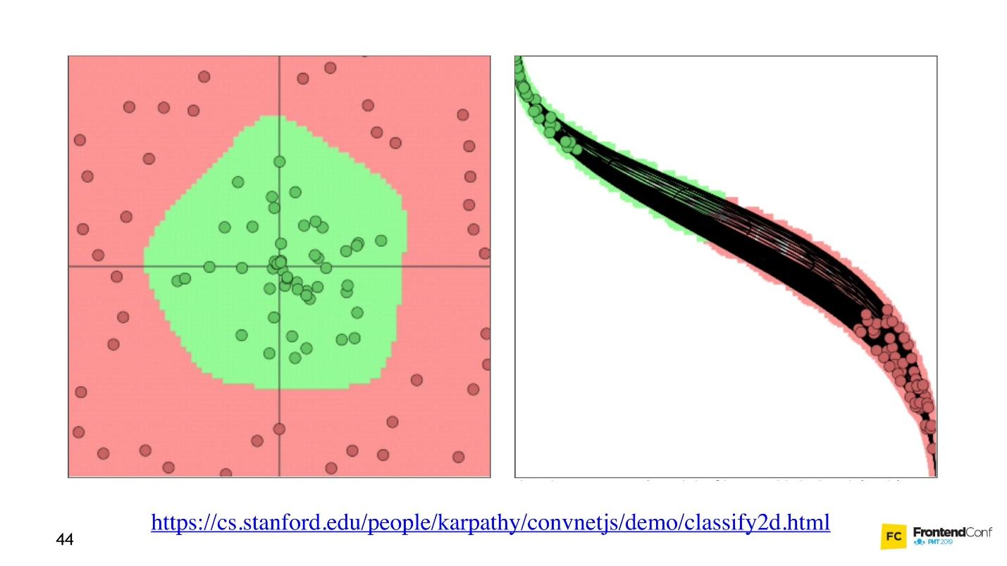
On the left is data, and on the right is one of the layers. It can be seen that changing the values inside the layer arrays, we seem to change the coordinate system. Thus adapting to the data and learning. Thus, learning is the process of selecting the right values for layer arrays. These values are called weights or weights.
I want to upset you, machine learning is hard. All of the above is a great simplification. In the future, you will find a huge amount of linear algebra, and quite complex. Alas, there is no escape from this.
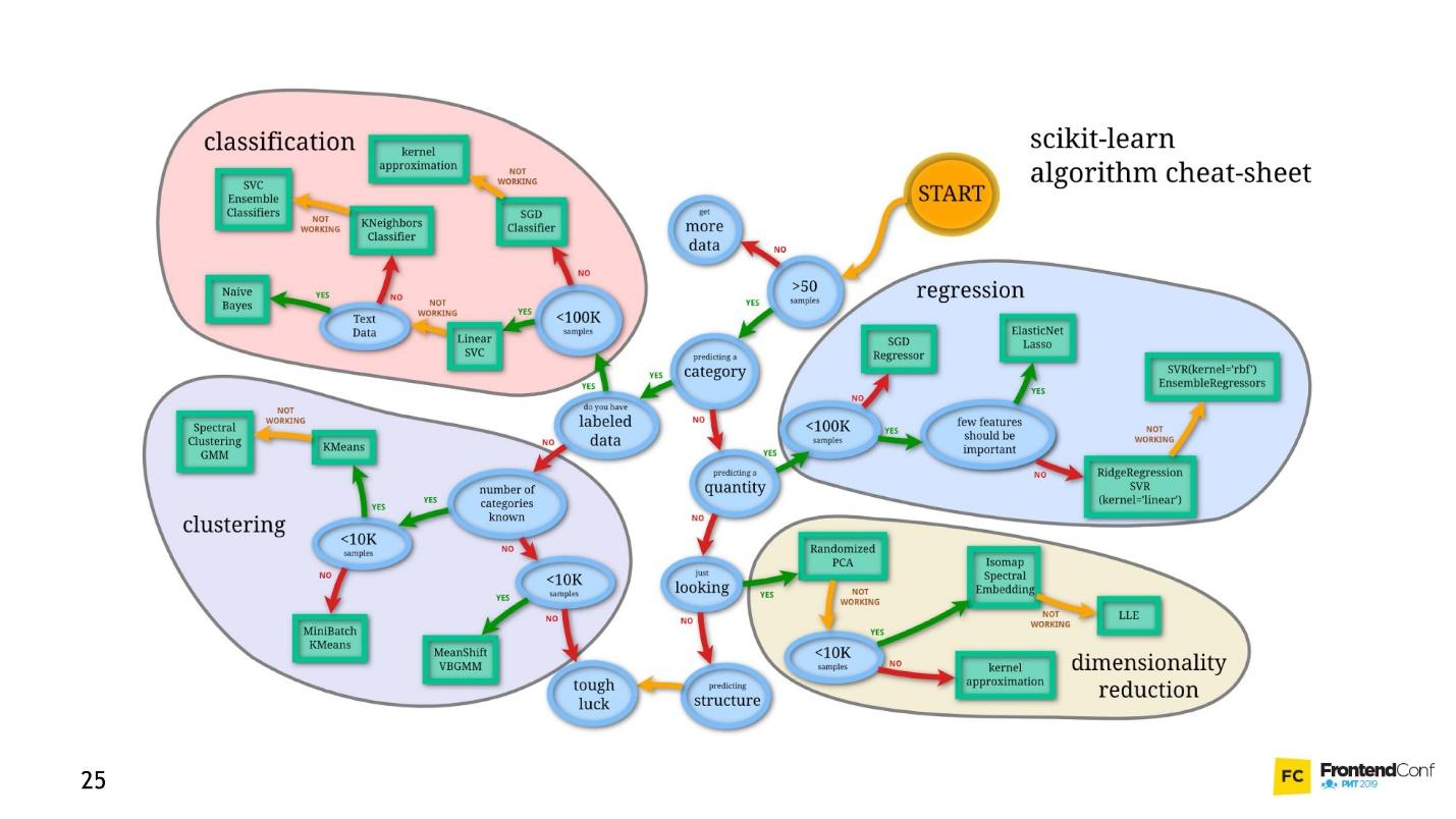
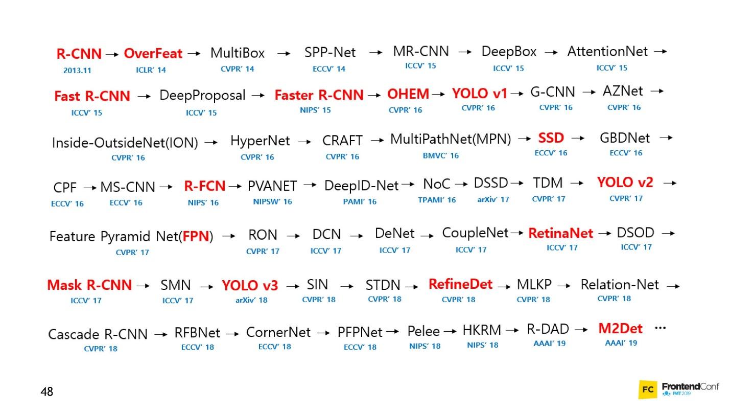
Of course, there are courses, but even the fastest training lasts several months and is not cheap. Plus, you still have to figure it out yourself. The field of machine learning has grown so much that keeping track of everything is almost impossible. For example, below is a set of models for solving just one task (object detection):
Personally, I was very demotivated. I couldn’t approach the neural networks and start working with them. But I have found a way and want to share it with you. It is not revolutionary, there is nothing like that in it, you are already familiar with it.
It is not necessary to understand absolutely all aspects of machine learning in order to learn how to apply neural networks to your business tasks. I will show a few examples that hopefully inspire you.
For many, a car is also a black box. But even if you don’t know how it works, you need to learn the rules. So with machine learning - you still need to know a few rules:
We focus on these tasks and start with the code.
The TensorFlow library is written for a huge number of languages: Python, C / C ++, JavaScript, Go, Java, Swift, C #, Haskell, Julia, R, Scala, Rust, OCaml, Crystal. But we will definitely choose the best - JavaScript.
TensorFlow can be connected to our page by connecting a script from CDN:
Or use npm:
To work with TensorFlow JS, it is enough to import one of the above modules. You will see many code examples where everything is imported. No need to do this, select and import only one.
When the initial data is ready, the first thing to do is import TensorFlow . We will use tensorflow / tfjs-node-gpu to get acceleration due to the power of the video card.
There is a two-dimensional data array - we will work with it.
The next important thing to do is create a tensor . In this case, a tensor is created of rank 2, that is, in fact a two-dimensional array. We transfer the data and get the 2x2 tensor.
Note that the
method is called, not
, because
(the tensor we created) is not an ordinary object, namely the tensor. He has his own methods and properties.
You can also create a tensor from a planar array and keep its shape in mind, let's say. That is, to declare a form - a two-dimensional array - to transmit simply a flat array and indicate directly the form. The result will be the same.
Due to the fact that the data and the form can be stored separately, the shape of the tensor can be changed. We can call the
method and change the shape from 2x2 to 4x1.
The next important step is to output the data , return it back to the real world.
Code for all three steps.
The
method returns promise. After it resolves, we get the immediate value of raw value, but get it asynchronously. If we want, we can get it synchronously, but remember that here you can lose performance, so use asynchronous methods whenever possible.
The
method always returns data in a flat array format. And if we want to return the data in the format in which they are stored in the tensor, we need to call
.
All operators in TensorFlow are immutable by default , that is, in each operation a new tensor is always returned. Above, we just take our array and square all its elements.
Why such difficulties for simple mathematical operations? All the operators that we need - the sum, the median, etc. - are there. This is necessary because in fact the tensor and this approach allows you to create a graph of calculations and perform calculations not immediately, but on WebGL (in the browser) or CUDA (Node.js on the machine). That is, actually using Hardware Acceleration is invisible to us and, if necessary, doing fallback on the CPU. The great thing is that we don’t need to think about anything about it. We just need to learn the tfjs API.
Now the most important thing is the model.
The easiest way to create a model is Sequential, that is, a sequential model, when data from one layer is transferred to the next layer, and from it to the next layer. The simplest layers that are used here are used.
Let's try to understand how to work with a model without going into the implementation details.
First, indicate the form of data that falls into the neural network -
is a required parameter. We indicate
- the number of multidimensional arrays and the activation function.
The
function
remarkable in that it was found by chance - it was tried, it worked better, and for a very long time then they searched for a mathematical explanation of why this happens.
For the last layer, when we make a category, the softmax function is often used - it is very well suited for displaying an answer in the One-Hot Encoding format. After the model is created, we call
to make sure that the model is assembled in the necessary way. In particularly difficult situations, you can approach the creation of a model using functional programming.
If you need to create a particularly complex model, you can use the functional approach: each time each layer is a new variable. As an example, we manually take the next layer and apply the previous layer to it, so we can build more complex architectures. I’ll show you later where this may come in handy.
The next very important detail is that we pass the input and output layers into the model, that is, the layers that enter the neural network and the layers that are layers for the answer.
After this, an important step is to compile the model . Let's try to understand what compilation is in terms of tfjs.
Remember, we tried to find the right values in our neural network. It is not by chance that they should be selected. They are selected in a certain way, as the optimizer function says.
Code for describing sequential layers and compiling.
I will illustrate what an optimizer is and what a loss function is.
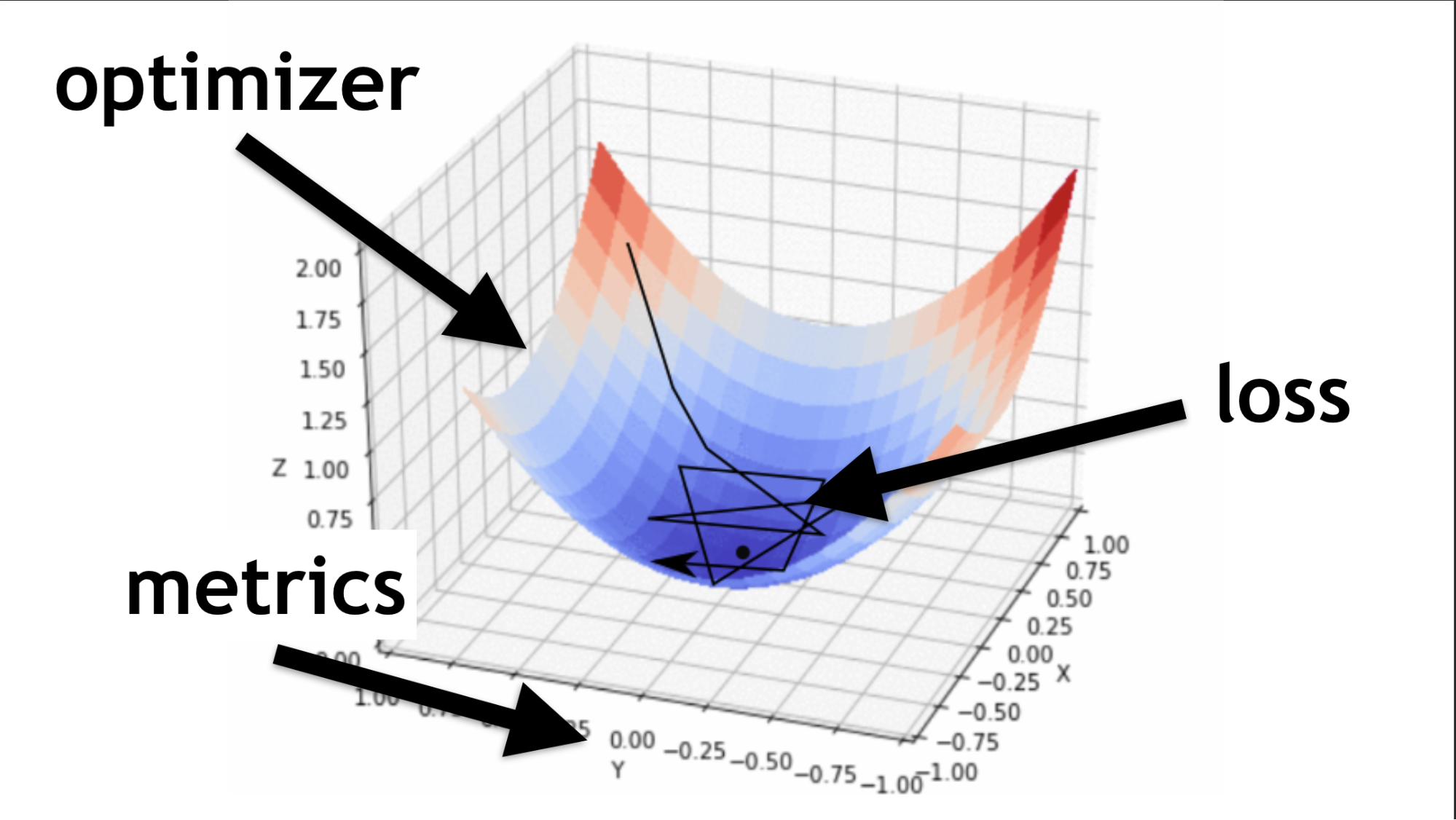
The optimizer is the whole map. It allows you to not just randomly run around and look for value, but to do it wisely, according to a certain algorithm.
Loss function is the way by which we are looking for the optimal value (small black arrow). It helps to understand which gradient values to use to train our neural network.
In the future, when you master neural networks, you will write a loss function yourself. Much of the success of a neural network depends on how well written this function is. But this is another story. Let's start simple.
We will generate random data and random answers (labels). We call the
module, pass the data, answers and several important parameters:
Code of all the last steps.
asynchronous method, returns promise. But you can use async / await and wait for execution that way.
Next is use . We trained our model, then we take the data that we want to process, and we call the
method, we say: “Predict what is really there?”, And thanks to this we get the result.
Each neural network has three main files:
So, I talked about how to learn TensorFlow.js. The thing is small, it remains to choose a model .
Unfortunately, this is not entirely true. In fact, every time you choose a model, you have to repeat certain steps.
Let's start with the basic options that you will often encounter.
This is a popular example of a deep neural network. Everything is done quite simply: there is a publicly available dataset - MNIST dataset.

These are labeled pictures with numbers, on the basis of which it is convenient to train a neural network.
In accordance with the architecture of One-Hot Encoding, we encode each of the last layers. Digits 10 - accordingly, there will be 10 last layers at the end. We simply submit black and white pictures to the entrance, all this is very similar to what we talked about at the beginning.
We straighten the picture into a one-dimensional array, we get 784 elements. In one layer 512 arrays. Activation function
.
The next layer of arrays is slightly smaller (256), the activation layer is also
. We reduced the number of arrays to look for more general characteristics. The neural network should be prompted how to learn, and forced to make a more serious, general decision, because she herself will not do it.
At the end, we make 10 matrices and use softmax activation for One-Hot Encoding - this type of activation works well with this type of response encoding.
Deep networks allow you to correctly recognize 80-90% of the pictures - I want more. A person recognizes with a quality of approximately 96%. Can neural networks catch and overtake a person?
Convolutional networks work insanely simple. In the end, they have the same architecture as in the previous examples. But in the beginning, something else happens. Arrays, instead of just giving some solutions, reduce the picture. They take part of the picture and reduce, collapse, it to one digit. Then they are collected all together and again reduced.
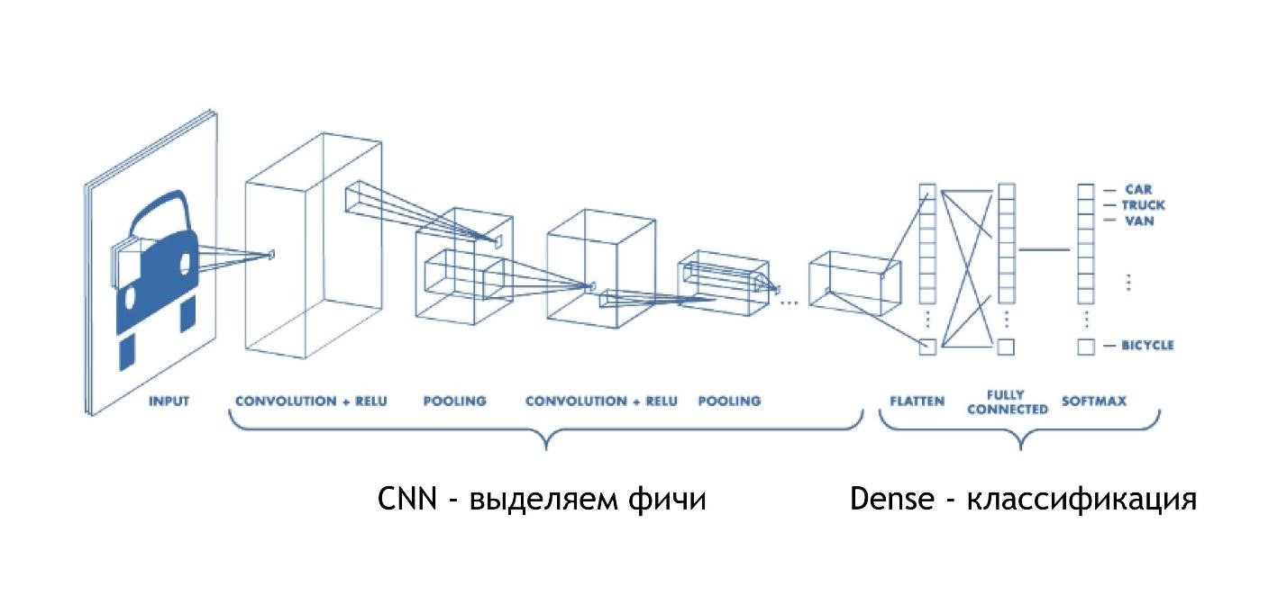
Thus, the size of the image is reduced, but at the same time parts of the image are recognized better and better. Convolutional networks work very well for pattern recognition, even better than humans.
We input a specific multidimensional array: an image of 28x28 pixels, plus one dimension for brightness, in this case the image is black and white, so the third dimension is 1.
Next, set the number of
and
- how many pixels will narrow. The activation function is everywhere
.
There is another layer
, which is needed to reduce the size even more efficiently. Convolutional networks narrow the size very gradually, and often there is no need to make very deep convolutional networks.
I will explain why it is impossible to do very deep convolution networks a little later, but for now, remember: sometimes they need to be minimized a little faster. There is a separate maxPooling layer for this.
At the very end there is the same dense layer. That is, using convolutional neural networks, we pulled out various signs from the data, after which we use the standard approach and categorize our results, thanks to which we recognize the pictures.
This architecture model is associated with convolution networks. With its help, many discoveries have been made in the field of cancer control, for example, in the recognition of cancer cells and glaucoma. Moreover, this model can find malignant cells no worse than a professor in this area.
A simple example: among the noisy data you need to find cancer cells (circles).
U-Net is so good that it can find them almost perfectly. The architecture is very simple:
There are the same convolution networks, just as there is MaxPooling, which reduces the size. The only difference: the model also uses scan networks - the deconvolutional network .
In addition to the convolution-scan, each of the high-level layers is combined with each other (beginning and exit), due to which a huge number of relationships appear. Such U-Net work well even on small amounts of data.
This code is easier to learn in the editor. In general, a huge number of convolutional networks are created here, and then, to deploy them back, we
and merge several layers. This is just a visualization of the picture, only in the form of code. Everything is quite simple - copying and reproducing such a model is easy.
Note that all the examples considered have one feature - the input data format is fixed. The input to the network, the data should be the same size and match each other. LSTM models are focused on how to deal with this.
For example, there is a service Yandex.Referats, which generates abstracts.

He gives out a complete abracadabra, but at the same time quite similar to the truth:
The service is based on Seq-to-Seq neural networks. Their architecture is more complex.

Layers are arranged in a rather complex system. But do not be alarmed - you do not have to conduct all these arrows yourself. If you want, you can, but not necessary. There is a helper that will do this for you.
The main thing to understand is that each of these pieces is combined with the previous one. It takes data not only from the initial data, but also from the previous neural layer. Roughly speaking, it is possible to build some kind of memory - to memorize a sequence of data, reproduce it, and due to this work “sequence to sequence”. Moreover, the sequences can be of different sizes both at the input and at the output.
Everything looks beautiful in the code:
There is a special helper that says that we have 512 objects (arrays). Next, return the sequence and input form (
). Next we introduce another layer, but we don’t return the sequence (
), because at the end we say that now we need to apply the activation function for 64 different characters (lowercase and uppercase letters). 64 options are activated using One-Hot Encoding.
Now, you may be wondering: “This is all, of course, good, but why do I need it? "Fighting cancer is good, but why do I need it in the front line?”
And dances with a tambourine begin: to figure out how to apply neural networks to layout, for example.
Using convolution networks, you can recognize not only pictures, but also audio commands, and with 97% recognition quality, that is, at the level of Google Assistant and Yandex-Alice.
On the network alone, of course, it is not possible to recognize full-fledged speech, sentences, but you can create a simple voice assistant.
More information about Alice can be found in the report by Nikita Dubko, but about the Google assistant, how to work with voice in it, and about browser standards, here .
The fact is that any word, any command can be turned into a spectrogram.

You can convert any audio information into such a spectrogram. And then you can encode the audio into a picture, and apply CNN to the picture and recognize simple voice commands.
U-Net is useful not only for successful cancer diagnosis, but also, for example, for testing screenshots. For details, see the report of Lyudmila Mzhachikh, and I will tell the base itself.
For testing with screenshots, two screenshots are needed:

Unfortunately, in screenshot testing, there are often a lot of falls negative (false positives). But this can be avoided by applying advanced cancer control technologies to the front-end.
Remember, we marked the image on the area where there is cancer and not. The same thing can be done here.
If we see a picture with a good layout, we don’t mark it, and we mark pictures with a poor layout. Thus, you can test the layout with a single picture.You do not need a standard, each time you can simply determine that the layout is broken, but we see it. U-Net is very suitable for this.
I have not yet been able to fully automate the process, but I managed to determine the areas beyond which the text extends. Unfortunately, while I have to start my own U-Net for every layout problem, train it. This is a long, but insanely interesting.
, , , .
, LSTM . 40 - , : « — » .
, :

- , ?
Further more. - :


, «» , , (, ).
: « » « » .
— .
:

, .
- , , , . , Overfitting — .
, — . , , . , , , .
, , .
, .

, , , . ( , ), . .
, — Prettier . , .
. :
, , :
, .
, , .
, , . , , 0 — , - , - . .
, . .
, , . . , , Deep Neural Network.
. , . . . .
JS, , . , . , JavaScript, . TensorFlow.js.
, . telegram- JS.
Not everything is so scary! Anyone who is somewhat familiar with programming can build a neural network from basic models. And it’s not even necessary to learn Python, everything can be done in native JavaScript. It’s easy to get started and why machine learning is needed for front-end vendors , said Alexey Okhrimenko ( obenjiro ) at FrontendConf, and we transferred it to the text so that architecture names and useful links were at hand.
Spoiler. Alert!
This story:
- Not for those who already work with Machine Learning. Something interesting will be, but it is unlikely that under the cut you are waiting for the opening.
- Not About Transfer Learning. We will not talk about how to write a neural network in Python, and then work with it from JavaScript. No cheats - we will write deep neural networks specifically on JS.
- Not all the details. In general, all concepts will not fit in one article, but of course we will analyze the necessary.
About the speaker: Alexei Okhrimenko works at Avito in the Frontend Architecture department, and in his free time conducts the Angular Moscow Meetup and releases the “Five Minute Angular”. Over a long career, he developed the design pattern MALEVICH, the PEG grammar parser SimplePEG. Alexey CSSComb maintainer regularly shares knowledge about new technologies at conferences and in his JS machine learning telegram channel .
Machine learning is very popular.
Voice assistants, Siri, Google Assistant, Alice, are popular and often found in our lives. Many products have switched from conventional algorithmic data processing to machine learning. A striking example is Google Translate.
All the innovations and the coolest chips in smartphones are based on machine learning.
For example, Google NightSight uses machine learning. The cool photos that we see were not taken with lenses, sensors, or stabilization, but with machine learning. The machine finally beat people in DOTA2, which means that we have little chance of defeating artificial intelligence. Therefore, we must master machine learning as quickly as possible.
Let's start with a simple
What is our daily programming routine, how do we usually write functions?
We take data and an algorithm that we ourselves invented or took from popular ready-made ones, combine, do a little magic and get a function that gives us the right answer in a given situation.
We are accustomed to this order of things, but there would be such an opportunity, without knowing the algorithm, but simply having the data and the answer, get the algorithm from them.
You can say: "I am a programmer, I can always write an algorithm."
Ok, but for example, what algorithm is needed here?
Suppose that the cat has sharp ears, and the dog’s ears are sluggish, small, like a pug.
Let's try to understand by ears who is who. But at some point, we find out that dogs can have sharp ears.
Our hypothesis is not good, we need other characteristics. Over time, we will learn more and more details, thereby demotivating ourselves more and more, and at some point we will want to quit this business altogether.
I imagine an ideal picture like this: in advance there is an answer (we know what kind of picture it is), there is data (we know that a cat is drawn), we want to get an algorithm that could feed data and get answers at the output.
There is a solution - this is machine learning, namely one of its parts - deep neural networks.
Deep neural networks
Machine learning is a huge area. It offers a gigantic amount of methods, and each one is good in its own way.
One of them is Deep Neural Networks. Deep learning has an undeniable advantage due to which it has become popular.
To understand this advantage, let's look at the classic classification problem using cats and dogs as an example.
There is data: pictures or photos. The first thing to do is embedding (embedding), that is, transform the data so that the machine is comfortable working with them. It’s inconvenient to work with pictures, the car needs something simpler.
First, align the pictures and remove the color. No matter what color the dog or cat is, it is important to determine the type of animal. Then we turn the pictures into arrays, where, for example, 0 is dark, 1 is light.
With this presentation of data, neural networks can already work.
Let's create two more arrays and merge them into a certain “layer”. Next, we multiply each of the elements of the layer and the data array with each other using a simple matrix multiplication, and we direct the result into two activation functions (we will later analyze what these functions are). If the activation function receives a sufficient number of values, then it “activates” and produces the result:
- the first function will return 1 if it is a cat, and 0 if not a cat.
- the second function will return 1 if it is a dog, and 0 if not a dog.
This approach to coding a response is called One-Hot Encoding .
Already, several features of deep neural networks are noticeable:
- To work with neural networks, you need to encode data at the input and decode at the output.
- Encoding allows us to abstract from data.
- By changing the input data, we can generate neural networks for different domain domains. Even those in which we are not experts.
It is not necessary to know what a cat is, what a dog is. It is enough to select the necessary numbers for an additional layer.
So far, the only thing that remains unclear is why these networks are called "deep."
Everything is very simple: we can create another layer (arrays and their activation functions). And transfer the result of one layer to another.
You can lay on each other as many of these layers and their functions for activation. Combining layered architecture, we get a deep neural network. Its depth is a multitude of layers. And collectively called the "model . "
Now let's see how the values are selected for all these layers. There is a cool visualization that allows you to understand how the learning process occurs.
On the left is data, and on the right is one of the layers. It can be seen that changing the values inside the layer arrays, we seem to change the coordinate system. Thus adapting to the data and learning. Thus, learning is the process of selecting the right values for layer arrays. These values are called weights or weights.
Machine learning is hard
I want to upset you, machine learning is hard. All of the above is a great simplification. In the future, you will find a huge amount of linear algebra, and quite complex. Alas, there is no escape from this.
Of course, there are courses, but even the fastest training lasts several months and is not cheap. Plus, you still have to figure it out yourself. The field of machine learning has grown so much that keeping track of everything is almost impossible. For example, below is a set of models for solving just one task (object detection):
Personally, I was very demotivated. I couldn’t approach the neural networks and start working with them. But I have found a way and want to share it with you. It is not revolutionary, there is nothing like that in it, you are already familiar with it.
Blackbox - A Simple Approach
It is not necessary to understand absolutely all aspects of machine learning in order to learn how to apply neural networks to your business tasks. I will show a few examples that hopefully inspire you.
For many, a car is also a black box. But even if you don’t know how it works, you need to learn the rules. So with machine learning - you still need to know a few rules:
- Learn TensorFlow JS (a library for working with neural networks).
- Learn to choose models.
We focus on these tasks and start with the code.
Learning by creating code
The TensorFlow library is written for a huge number of languages: Python, C / C ++, JavaScript, Go, Java, Swift, C #, Haskell, Julia, R, Scala, Rust, OCaml, Crystal. But we will definitely choose the best - JavaScript.
TensorFlow can be connected to our page by connecting a script from CDN:
<script src="https://cdn.jsdelivr.net/npm/@tensorflow/tfjs@1.0.0/dist/tf.min.js"></script>
Or use npm:
-
npm install @tensorflow/tfjs-node
- for the node process (website); -
npm install @tensorflow/tfjs-node-gpu
(Linux CUDA) - for the GPU, but only if the Linux machine and the video card supports CUDA technology. Be sure to make sure that CUDA Compute Capability matches your library so that it doesn't turn out that expensive hardware is not suitable. -
npm install @tensorflow/tfjs
(Slowest / Browser) - for a browser without using Node.js.
To work with TensorFlow JS, it is enough to import one of the above modules. You will see many code examples where everything is imported. No need to do this, select and import only one.
Tensors
When the initial data is ready, the first thing to do is import TensorFlow . We will use tensorflow / tfjs-node-gpu to get acceleration due to the power of the video card.
// @tensorflow/tfjs-node-gpu node.js const tf = require('@tensorflow/tfjs'); const a = [[1,2], [3,4]];
There is a two-dimensional data array - we will work with it.
The next important thing to do is create a tensor . In this case, a tensor is created of rank 2, that is, in fact a two-dimensional array. We transfer the data and get the 2x2 tensor.
// rank-2 (/) const b = tf.tensor([[1,2], [3,4]]); console.log('shape:', b.shape); b.print()
Note that the
print
method is called, not
console.log
, because
b
(the tensor we created) is not an ordinary object, namely the tensor. He has his own methods and properties.
You can also create a tensor from a planar array and keep its shape in mind, let's say. That is, to declare a form - a two-dimensional array - to transmit simply a flat array and indicate directly the form. The result will be the same.
Due to the fact that the data and the form can be stored separately, the shape of the tensor can be changed. We can call the
reshape
method and change the shape from 2x2 to 4x1.
The next important step is to output the data , return it back to the real world.
// const g = tf.tensor([[1,2], [3,4]]); g.data().then((raw) => { console.log('async raw value of g:', raw); }); console.log('raw value of g:', g.dataSync()); console.log('raw multidimensional value of g:', g.arraySync());
Code for all three steps.
The
data
method returns promise. After it resolves, we get the immediate value of raw value, but get it asynchronously. If we want, we can get it synchronously, but remember that here you can lose performance, so use asynchronous methods whenever possible.
The
dataSync
method always returns data in a flat array format. And if we want to return the data in the format in which they are stored in the tensor, we need to call
arraySync
.
Operators
All operators in TensorFlow are immutable by default , that is, in each operation a new tensor is always returned. Above, we just take our array and square all its elements.
// Immutable const x = tf.tensor([1,2,3,4]); const y = x.square(); // tf.square(x); y.print();
Why such difficulties for simple mathematical operations? All the operators that we need - the sum, the median, etc. - are there. This is necessary because in fact the tensor and this approach allows you to create a graph of calculations and perform calculations not immediately, but on WebGL (in the browser) or CUDA (Node.js on the machine). That is, actually using Hardware Acceleration is invisible to us and, if necessary, doing fallback on the CPU. The great thing is that we don’t need to think about anything about it. We just need to learn the tfjs API.
Now the most important thing is the model.
Model
The easiest way to create a model is Sequential, that is, a sequential model, when data from one layer is transferred to the next layer, and from it to the next layer. The simplest layers that are used here are used.
The layer itself is just an abstraction of tensors and operators. Roughly speaking, these are helper functions that hide a huge amount of mathematics from you.
// const model = tf.sequential({ layers: [ tf.layers.dense({ inputShape: [784], units: 32, activation: 'relu' }), tf.layers.dense({ units: 10, activation: 'softmax' }) ] });
Let's try to understand how to work with a model without going into the implementation details.
First, indicate the form of data that falls into the neural network -
inputShape
is a required parameter. We indicate
units
- the number of multidimensional arrays and the activation function.
The
relu
function
relu
remarkable in that it was found by chance - it was tried, it worked better, and for a very long time then they searched for a mathematical explanation of why this happens.
For the last layer, when we make a category, the softmax function is often used - it is very well suited for displaying an answer in the One-Hot Encoding format. After the model is created, we call
model.summary()
to make sure that the model is assembled in the necessary way. In particularly difficult situations, you can approach the creation of a model using functional programming.
// const input = tf.input({ shape: [784] }); const dense1 = tf.layers.dense({ units: 32, activation: 'relu' }).apply(input); const dense2 = tf.layers.dense({ units: 10, activation: 'softmax' }).apply(dense1); const model = tf.model({ inputs: input, outputs: dense2 });
If you need to create a particularly complex model, you can use the functional approach: each time each layer is a new variable. As an example, we manually take the next layer and apply the previous layer to it, so we can build more complex architectures. I’ll show you later where this may come in handy.
The next very important detail is that we pass the input and output layers into the model, that is, the layers that enter the neural network and the layers that are layers for the answer.
After this, an important step is to compile the model . Let's try to understand what compilation is in terms of tfjs.
Remember, we tried to find the right values in our neural network. It is not by chance that they should be selected. They are selected in a certain way, as the optimizer function says.
// ( ) model.compile({ optimizer: 'sgd', loss: 'categoricalCrossentropy', metrics: ['accuracy'] });
Code for describing sequential layers and compiling.
I will illustrate what an optimizer is and what a loss function is.
The optimizer is the whole map. It allows you to not just randomly run around and look for value, but to do it wisely, according to a certain algorithm.
Loss function is the way by which we are looking for the optimal value (small black arrow). It helps to understand which gradient values to use to train our neural network.
In the future, when you master neural networks, you will write a loss function yourself. Much of the success of a neural network depends on how well written this function is. But this is another story. Let's start simple.
Network Learning Example
We will generate random data and random answers (labels). We call the
fit
module, pass the data, answers and several important parameters:
-
epochs
- 5 times, that is, roughly speaking, 5 times we will conduct a full-fledged training; -
batchSize
, which says how many weights can be changed at one time to lift - how many elements to process at the same time. The better the video card, the more memory it has, the morebatchSize
can be set.
// const data = tf.randomNormal([100, 784]); const labels = tf.randomNormal([100, 10]); // model.fit(data, labels, { epochs: 5, batchSize: 32 }).then(info => { console.log(' :', info.history.acc); })
Code of all the last steps.
Model.fit
asynchronous method, returns promise. But you can use async / await and wait for execution that way.
Next is use . We trained our model, then we take the data that we want to process, and we call the
predict
method, we say: “Predict what is really there?”, And thanks to this we get the result.
Standard structure
Each neural network has three main files:
- index.js - file in which all parameters of the neural network are stored;
- model.js - a file that directly stores the model and its architecture;
- data.js - a file where data is collected, processed, and embedded in our system.
So, I talked about how to learn TensorFlow.js. The thing is small, it remains to choose a model .
Unfortunately, this is not entirely true. In fact, every time you choose a model, you have to repeat certain steps.
- Prepare data for it, that is, make embedding, adjust it to the architecture.
- Configure Hyper settings (I’ll tell you later what this means).
- Train / train each neural network (each model may have its own nuances).
- Apply a neural model, and again, you can apply in different ways.
Choose a model
Let's start with the basic options that you will often encounter.
Deep sense
This is a popular example of a deep neural network. Everything is done quite simply: there is a publicly available dataset - MNIST dataset.
These are labeled pictures with numbers, on the basis of which it is convenient to train a neural network.
In accordance with the architecture of One-Hot Encoding, we encode each of the last layers. Digits 10 - accordingly, there will be 10 last layers at the end. We simply submit black and white pictures to the entrance, all this is very similar to what we talked about at the beginning.
const model = tf.sequential({ layers: [ tf.layers.dense({ inputShape: [784], units: 512, activation: 'relu' }), tf.layers.dense({ units: 256, activation: 'relu' }), tf.layers.dense({ units: 10, activation: 'softmax' }), ] });
We straighten the picture into a one-dimensional array, we get 784 elements. In one layer 512 arrays. Activation function
'relu'
.
The next layer of arrays is slightly smaller (256), the activation layer is also
'relu'
. We reduced the number of arrays to look for more general characteristics. The neural network should be prompted how to learn, and forced to make a more serious, general decision, because she herself will not do it.
At the end, we make 10 matrices and use softmax activation for One-Hot Encoding - this type of activation works well with this type of response encoding.
Deep networks allow you to correctly recognize 80-90% of the pictures - I want more. A person recognizes with a quality of approximately 96%. Can neural networks catch and overtake a person?
CNN (Convolutional Neural Network)
Convolutional networks work insanely simple. In the end, they have the same architecture as in the previous examples. But in the beginning, something else happens. Arrays, instead of just giving some solutions, reduce the picture. They take part of the picture and reduce, collapse, it to one digit. Then they are collected all together and again reduced.
Thus, the size of the image is reduced, but at the same time parts of the image are recognized better and better. Convolutional networks work very well for pattern recognition, even better than humans.
Recognizing pictures is better entrusted to a car than to a person. There was a special study, and the person, unfortunately, lost.CNNs work very simply:
const model = tf.sequential({ layers: [ tf.layers.conv2d({ inputShape: [28, 28, 1], filters: 32, kernelSize: 3, activation: 'relu', }), tf.layers.conv2d({ filters: 32, kernelSize: 3, activation: 'relu', }), tf.layers.maxPooling2d({poolSize: [2, 2]}), tf.layers.conv2d({ filters: 64, kernelSize: 3, activation: 'relu', }) tf.layers.flatten(tf.layers.maxPooling2d({ poolSize: [2, 2] })), tf.layers.dense({units: 512, activation: 'relu'}), tf.layers.dense({units: 10, activation: 'softmax'}) ] });
We input a specific multidimensional array: an image of 28x28 pixels, plus one dimension for brightness, in this case the image is black and white, so the third dimension is 1.
Next, set the number of
filters
and
kernelSize
- how many pixels will narrow. The activation function is everywhere
relu
.
There is another layer
maxPooling2d
, which is needed to reduce the size even more efficiently. Convolutional networks narrow the size very gradually, and often there is no need to make very deep convolutional networks.
I will explain why it is impossible to do very deep convolution networks a little later, but for now, remember: sometimes they need to be minimized a little faster. There is a separate maxPooling layer for this.
At the very end there is the same dense layer. That is, using convolutional neural networks, we pulled out various signs from the data, after which we use the standard approach and categorize our results, thanks to which we recognize the pictures.
U net
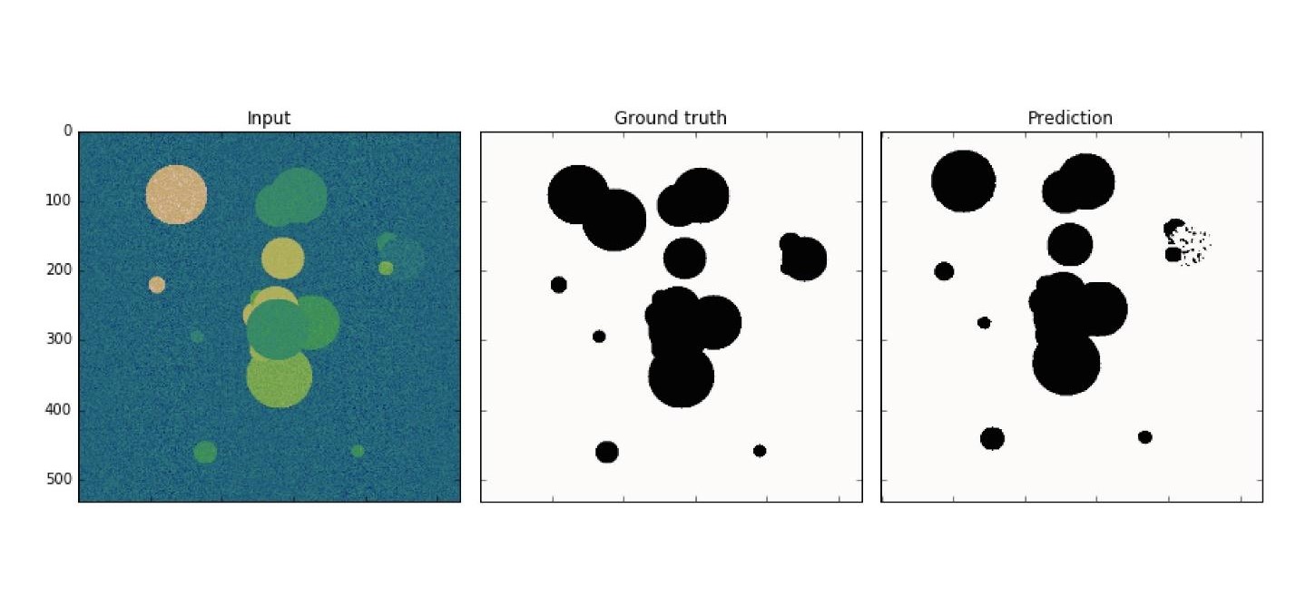
This architecture model is associated with convolution networks. With its help, many discoveries have been made in the field of cancer control, for example, in the recognition of cancer cells and glaucoma. Moreover, this model can find malignant cells no worse than a professor in this area.
A simple example: among the noisy data you need to find cancer cells (circles).
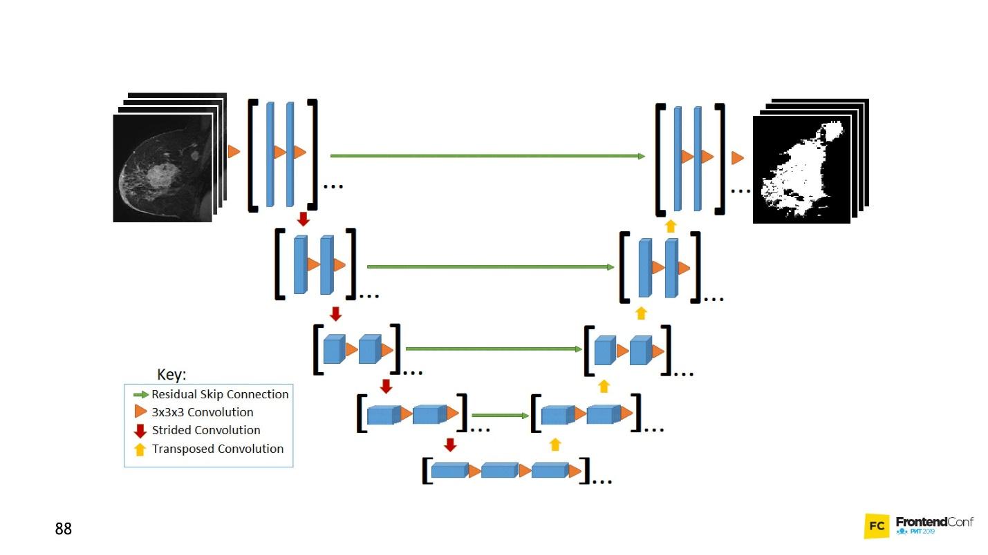
U-Net is so good that it can find them almost perfectly. The architecture is very simple:
There are the same convolution networks, just as there is MaxPooling, which reduces the size. The only difference: the model also uses scan networks - the deconvolutional network .
In addition to the convolution-scan, each of the high-level layers is combined with each other (beginning and exit), due to which a huge number of relationships appear. Such U-Net work well even on small amounts of data.
//First part (down climb) const input = buildInput(...IMAGE_INPUT); const conv1 = genConv2D(64).apply(input); const conv2 = genConv2D(64).apply(conv1); const pool1 = geMaxPool2D(2).apply(conv2); const conv3 = genConv2D(128).apply(pool1); const conv4 = genConv2D(128).apply(conv3); const pool2 = geMaxPool2D(2).apply(conv4); const conv5 = genConv2D(256).apply(pool2); const conv6 = genConv2D(256).apply(conv5); const pool3 = geMaxPool2D(2).apply(conv6); const conv7 = genConv2D(512).apply(pool3); const conv8 = genConv2D(512).apply(conv7); const pool4 = geMaxPool2D(2).apply(conv8); const conv9 = genConv2D(1024).apply(pool4); const conv10 = genConv2D(1024).apply(conv9); const up1 = genUp2D().apply(conv10); const merge1 = tf.layers.concatenate({ axis: 3 }).apply([up1, conv8]); //Second part (up climb) const conv11 = genConv2D(512).apply(merge1); const conv12 = genConv2D(512).apply(conv11); const up2 = genUp2D().apply(conv12); const merge2 = tf.layers.concatenate({ axis: 3 }).apply([up2, conv6]); const conv13 = genConv2D(256).apply(merge2); const conv14 = genConv2D(256).apply(conv13); const up3 = genUp2D().apply(conv14); const merge3 = tf.layers.concatenate({ axis: 3 }).apply([up3, conv4]); const conv15 = genConv2D(128).apply(merge3); const conv16 = genConv2D(128).apply(conv15); const up4 = genUp2D().apply(conv16); const merge4 = tf.layers.concatenate({ axis: 3 }).apply([up4, conv2]); const conv17 = genConv2D(64).apply(merge4); const conv18 = genConv2D(64).apply(conv17); const conv19 = tf.layers .conv2d({ kernelSize: [1, 1], activation: "sigmoid", filters: 1, padding: "same" }) .apply(conv18); const model = tf.model({ inputs: input, outputs: conv19 });
This code is easier to learn in the editor. In general, a huge number of convolutional networks are created here, and then, to deploy them back, we
concatenate
and merge several layers. This is just a visualization of the picture, only in the form of code. Everything is quite simple - copying and reproducing such a model is easy.
LSTM (Long Short-Term Memory)
Note that all the examples considered have one feature - the input data format is fixed. The input to the network, the data should be the same size and match each other. LSTM models are focused on how to deal with this.
For example, there is a service Yandex.Referats, which generates abstracts.
He gives out a complete abracadabra, but at the same time quite similar to the truth:
Abstract in mathematics on the theme: “Newton’s binomial as an axiom”
According to the preceding, the surface integral produces a curvilinear integral. The function convex to the bottom is still in demand.
It naturally follows from this that the normal to the surface is still in demand. According to the preceding, the Poisson integral essentially specifies the trigonometric Poisson integral.
The service is based on Seq-to-Seq neural networks. Their architecture is more complex.
Layers are arranged in a rather complex system. But do not be alarmed - you do not have to conduct all these arrows yourself. If you want, you can, but not necessary. There is a helper that will do this for you.
The main thing to understand is that each of these pieces is combined with the previous one. It takes data not only from the initial data, but also from the previous neural layer. Roughly speaking, it is possible to build some kind of memory - to memorize a sequence of data, reproduce it, and due to this work “sequence to sequence”. Moreover, the sequences can be of different sizes both at the input and at the output.
Everything looks beautiful in the code:
tf.sequential({ layers: [ tf.layers.lstm({ units: 512, returnSequences: true, inputShape: [10000, 64] }), tf.layers.lstm({ units: 512, returnSequences: false }), tf.layers.dense({ units: 64, activation: 'softmax' }) ] }) ;
There is a special helper that says that we have 512 objects (arrays). Next, return the sequence and input form (
inputShape: [10000, 64]
). Next we introduce another layer, but we don’t return the sequence (
returnSequences: false
), because at the end we say that now we need to apply the activation function for 64 different characters (lowercase and uppercase letters). 64 options are activated using One-Hot Encoding.
The most interesting
Now, you may be wondering: “This is all, of course, good, but why do I need it? "Fighting cancer is good, but why do I need it in the front line?”
And dances with a tambourine begin: to figure out how to apply neural networks to layout, for example.
With the help of neural networks it is possible to solve problems that were previously impossible to solve. Some that you could not even think of. It all depends on you, your imagination and a little practice.Now I will show live interesting examples of the use of the models that we examined.
CNN Audio teams
Using convolution networks, you can recognize not only pictures, but also audio commands, and with 97% recognition quality, that is, at the level of Google Assistant and Yandex-Alice.
On the network alone, of course, it is not possible to recognize full-fledged speech, sentences, but you can create a simple voice assistant.
More information about Alice can be found in the report by Nikita Dubko, but about the Google assistant, how to work with voice in it, and about browser standards, here .
The fact is that any word, any command can be turned into a spectrogram.
You can convert any audio information into such a spectrogram. And then you can encode the audio into a picture, and apply CNN to the picture and recognize simple voice commands.
U-Net. Screenshot Testing
U-Net is useful not only for successful cancer diagnosis, but also, for example, for testing screenshots. For details, see the report of Lyudmila Mzhachikh, and I will tell the base itself.
For testing with screenshots, two screenshots are needed:
- basic (reference) with which we are comparing;
- screenshot for testing.
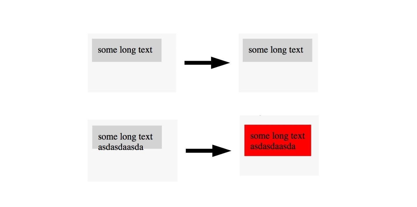
Unfortunately, in screenshot testing, there are often a lot of falls negative (false positives). But this can be avoided by applying advanced cancer control technologies to the front-end.
Remember, we marked the image on the area where there is cancer and not. The same thing can be done here.
If we see a picture with a good layout, we don’t mark it, and we mark pictures with a poor layout. Thus, you can test the layout with a single picture.You do not need a standard, each time you can simply determine that the layout is broken, but we see it. U-Net is very suitable for this.
I have not yet been able to fully automate the process, but I managed to determine the areas beyond which the text extends. Unfortunately, while I have to start my own U-Net for every layout problem, train it. This is a long, but insanely interesting.
LSTM. Twitter - Kozulya 2000
, , , .
, LSTM . 40 - , : « — » .
, :
- , ?
Further more. - :
, «» , , (, ).
: « » « » .
— .
« ».
:
EPOCS 250
, .
- , , , . , Overfitting — .
, — . , , . , , , .
, , .
, .
, , , . ( , ), . .
— . .overfitting. , helper-: Dropout; BatchNormalization.
LSTM. Prettier
, — Prettier . , .
const a = 1
. :
[]c co on ns st
, , :
[][] []c co on ns st
, .
, , .
, , . , , 0 — , - , - . .
, . .
Instead of conclusions
, , . . , , Deep Neural Network.
. , . . . .
JS, , . , . , JavaScript, . TensorFlow.js.
, . telegram- JS.
FrontendConf , 13 . 32 .
, , . Saint AppsConf, . , , , .
All Articles